wannier.c

Wannier flow between rotating excentric cylinders

Wannier flow between rotating excentric cylinders

This test case is similar to the Couette flow test case but we use here eccentric cylinders. While the concentric cylinders case can be reduced to a one-dimensional equation in polar coordinates (the radial velocity component vanishes), this is not the case for eccentric cylinders. For this problem (also known as “journal bearing” flow), an exact analytical solution in the limit of Stokes flows was obtained by Wannier, 1950 using conformal mapping.

#include "../myembed.h"
#if CENTERED == 1
#include "../mycentered2.h"
#else
#include "../mycentered.h"
#endif // CENTERED
#include "view.h"

Exact solution

We define here the exact solution, as computed by Wannier and evaluated at the center of each cell.

void psiuv (double x, double y, 
	    double r1, double r2, double e,
	    double v1, double v2,
	    double * ux, double * uy, double * psi)
{
  double d1 = (r2*r2 - r1*r1)/(2.*e) - e/2.;
  double d2 = d1 + e;
  double s = sqrt((r2 - r1 - e)*(r2 - r1 + e)*(r2 + r1 + e)*(r2 + r1 - e))
    /(2.*e);
  double l1 = log((d1 + s)/(d1 - s));
  double l2 = log((d2 + s)/(d2 - s));
  double den = (r2*r2 + r1*r1)*(l1 - l2) - 4.*s*e;
  double curlb = 2.*(d2*d2 - d1*d1)*(r1*v1 + r2*v2)/((r2*r2 + r1*r1)*den) +
    r1*r1*r2*r2*(v1/r1 - v2/r2)/(s*(r1*r1 + r2*r2)*(d2 - d1));
  double A = -0.5*(d1*d2-s*s)*curlb;
  double B = (d1 + s)*(d2 + s)*curlb;
  double C = (d1 - s)*(d2 - s)*curlb;
  double D = (d1*l2 - d2*l1)*(r1*v1 + r2*v2)/den
    - 2.*s*((r2*r2 - r1*r1)/(r2*r2 + r1*r1))*(r1*v1 + r2*v2)/den
    - r1*r1*r2*r2*(v1/r1 - v2/r2)/((r1*r1 + r2*r2)*e);
  double E = 0.5*(l1 - l2)*(r1*v1 + r2*v2)/den;
  double F = e*(r1*v1 + r2*v2)/den;

  y += d2;
  double spy = s + y;
  double smy = s - y;
  double zp = x*x + spy*spy;
  double zm = x*x + smy*smy;
  double l = log(zp/zm);
  double zr = 2.*(spy/zp + smy/zm);

  *psi = A*l + B*y*spy/zp + C*y*smy/zm + D*y + E*(x*x + y*y + s*s) + F*y*l;
  *ux = -A*zr - B*((s + 2.*y)*zp - 2.*spy*spy*y)/(zp*zp) -
    C*((s - 2.*y)*zm + 2.*smy*smy*y)/(zm*zm) - D -
    E*2.*y - F*(l + y*zr);
  *uy = -A*8.*s*x*y/(zp*zm) - B*2.*x*y*spy/(zp*zp) -
    C*2.*x*y*smy/(zm*zm) + E*2.*x -
    F*8.*s*x*y*y/(zp*zm);
}

We also define the shape of the domain. The strange choices for radii R1, R2 and eccentricity ECC come from the ‘bipolar’ variant.

#define R1 (1./sinh(1.5)) // 0.47
#define R2 (1./sinh(1.)) // 0.85
#define X1 (1./tanh(1.5))
#define X2 (1./tanh(1.))
#define ECC ((X2) - (X1)) // 0.21

void p_shape (scalar c, face vector f)
{
  vertex scalar phi[];
  foreach_vertex()
    phi[] = difference (sq (R2) - sq (x) - sq (y - (ECC)),
			sq (R1) - sq (x) - sq (y));
  fractions (phi, c, f);
  fractions_cleanup (c, f,
		     smin = 1.e-14, cmin = 1.e-14);
}

#if TREE

When using TREE, we try to increase the accuracy of the restriction operation in pathological cases by defining the gradient of u at the center of the cell. In this case, I was “lazy” and did not do it.

#endif // TREE

Setup

We need a field for viscosity so that the embedded boundary metric can be taken into account.

face vector muv[];

We also define a reference velocity field.

scalar un[];

int lvl;

int main()
{

The domain is 2.5\times 2.5.

  L0 = 2.5;
  size (L0);
  origin (-L0/2., -L0/2.);

We set the maximum timestep.

  DT = 1.e-2;

We set the tolerance of the Poisson solver.

  stokes       = true;
  TOLERANCE    = 1.e-5;
  TOLERANCE_MU = 1.e-5;

  for (lvl = 5; lvl <= 9; lvl++) { // minlevel = 3 (1.3pt/(R2 - R1 - ECC))

We initialize the grid.

    N = 1 << (lvl);
    init_grid (N);

    run();
  }
}

Boundary conditions

Properties

event properties (i++)
{
  foreach_face()
    muv.x[] = fm.x[];
}

Initial conditions

event init (i = 0)
{

We set the viscosity field in the event properties.

  mu = muv;

We use “third-order” face flux interpolation.

#if ORDER2
  for (scalar s in {u, p})
    s.third = false;
#else
  for (scalar s in {u, p})
    s.third = true;
#endif // ORDER2
  
#if TREE

When using TREE and in the presence of embedded boundaries, we should also define the gradient of u at the cell center of cut-cells.

#endif // TREE

We initialize the embedded boundary.

#if TREE

When using TREE, we refine the mesh around the embedded boundary.

  astats ss;
  int ic = 0;
  do {
    ic++;
    p_shape (cs, fs);
    ss = adapt_wavelet ({cs}, (double[]) {1.e-30},
  		       maxlevel = (lvl), minlevel = (lvl) - 2);
  } while ((ss.nf || ss.nc) && ic < 100);
#endif // TREE
  
  p_shape (cs, fs);

We also define the volume fraction at the previous timestep csm1=cs.

  csm1 = cs;

We define the boundary conditions for the velocity. The outer cylinder is fixed and the inner cylinder is rotating with an angular velocity \omega = 1.

  u.n[embed] = dirichlet (x*x + y*y > 1.5*sq(R1) ? 0. : - y/R1);
  u.t[embed] = dirichlet (x*x + y*y > 1.5*sq(R1) ? 0. :   x/R1);
  p[embed]   = neumann (0);
  
  uf.n[embed] = dirichlet (x*x + y*y > 1.5*sq(R1) ? 0. : - y/R1);
  uf.t[embed] = dirichlet (x*x + y*y > 1.5*sq(R1) ? 0. :   x/R1);

We finally initialize the reference velocity field.

  foreach()
    un[] = u.y[];
}

Embedded boundaries

Outputs

event error (i++; i <= 1000)
{

We look for a stationary solution.

  double du = change (u.y, un);
  if (i > 0 && du < 1e-5)
    return 1; /* stop */
}

event logfile (t = end)
{

The total (e), partial cells (ep) and full cells (ef) errors fields and their norms are computed.

  scalar nu[], e[], ep[], ef[];
  foreach() {
    if (cs[] == 0.)
      nu[] = ep[] = ef[] = e[] = nodata;
    else {
      double pw, uw, vw;
      psiuv (x, y - ECC, R1, R2, ECC, 1., 0., &uw, &vw, &pw);
      nu[] = sqrt (sq(u.x[]) + sq(u.y[]));
      e[]  = fabs (nu[] - sqrt(uw*uw + vw*vw));
      ep[] = cs[] < 1. ? e[] : nodata;
      ef[] = cs[] >= 1. ? e[] : nodata;
    }
  }
  norm n = normf (e), np = normf (ep), nf = normf (ef);
  
  fprintf (stderr, "%d %.3g %.3g %.3g %.3g %.3g %.3g %d %g %g %d %d %d %d\n",
	   N,
	   n.avg, n.max,
	   np.avg, np.max,
	   nf.avg, nf.max,
	   i, t, dt,
	   mgp.i, mgp.nrelax, mgu.i, mgu.nrelax);
  fflush (stderr);

  if (lvl == 5) {
    view (fov = 13.85, tx = 0, ty = -0.088);
    
    draw_vof ("cs", "fs", filled = -1, fc = {1,1,1});
    cells ();
    save ("mesh.png");

    draw_vof ("cs", "fs", filled = -1, fc = {1,1,1});
    squares ("nu", spread = -1);
    save ("nu.png");

    draw_vof ("cs", "fs", filled = -1, fc = {1,1,1});
    squares ("p", spread = -1);
    save ("p.png");

    draw_vof ("cs", "fs", filled = -1, fc = {1,1,1});
    squares ("e", spread = -1);
    save ("e.png");
    
    foreach() {
      double pw, uw, vw;
      psiuv (x, y, R1, R2, ECC, 1., 0., &uw, &vw, &pw);
      fprintf (stdout, "%g %g %g %g %g %g %g %g\n",
	       x, y,
	       u.x[], u.y[], p[],
	       e[], uw, vw);
      fflush (stdout);
    }
  }
}

Results

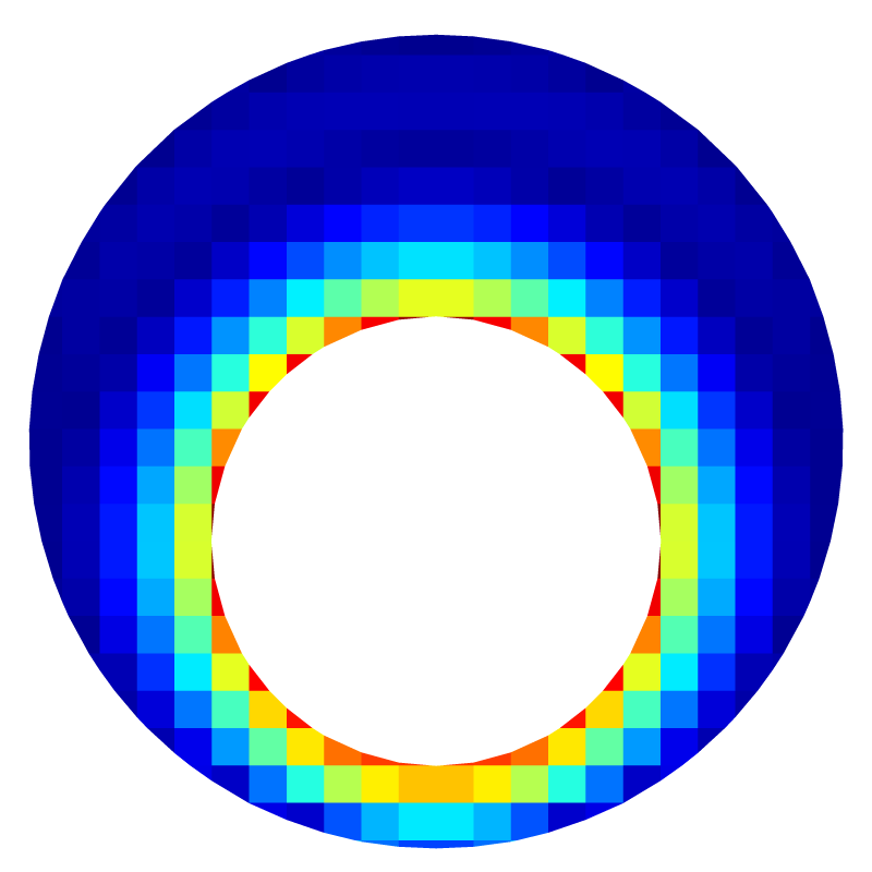
Norm of the velocity for l=5

The pressure field is not trivial.

Pressure field for l=5

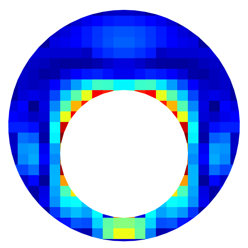
Error field for l=5

Errors

reset
set terminal svg font ",16"
set key bottom left spacing 1.1
set xtics 16,4,1024
set grid ytics
set ytics format "%.0e" 1.e-12,100,1.e2
set xlabel 'N'
set ylabel '||error||_{1}'
set xrange [16:1024]
set yrange [1.e-6:1.e-1]
set logscale
plot 'log' u 1:4 w p ps 1.25 pt 7 lc rgb "black" t 'cut-cells', \
     ''    u 1:6 w p ps 1.25 pt 5 lc rgb "blue" t 'full cells', \
     ''    u 1:2 w p ps 1.25 pt 2 lc rgb "red" t 'all cells'

Average error convergence (script)

set ylabel '||error||_{inf}'
plot '' u 1:5 w p ps 1.25 pt 7 lc rgb "black" t 'cut-cells', \
     '' u 1:7 w p ps 1.25 pt 5 lc rgb "blue" t 'full cells', \
     '' u 1:3 w p ps 1.25 pt 2 lc rgb "red" t 'all cells'

Maximum error convergence (script)

Order of convergence

We recover here the expected second-order convergence on a uniform grid. When using an adaptive grid, since the geometry of the outter cylinder is “convex”, pathological restriction operations (only 2 cells or less for the restriction operation) are more likely to occur. Since we have not defined the gradient of u to make these pathological restriction operations second-order, the convergence on an adaptive mesh is only first order.

reset
set terminal svg font ",16"
set key bottom left spacing 1.1
set xtics 16,4,1024
set ytics -4,2,4
set grid ytics
set xlabel 'N'
set ylabel 'Order of ||error||_{1}'
set xrange [16:1024]
set yrange [-4:4.5]
set logscale x

# Asymptotic order of convergence

ftitle(b) = sprintf(", asymptotic order n=%4.2f", -b);
Nmin = log(256);

f1(x) = a1 + b1*x; # cut-cells
f2(x) = a2 + b2*x; # full cells
f3(x) = a3 + b3*x; # all cells

fit [Nmin:*][*:*] f1(x) '< sort -k 1,1n log | awk "!/#/{print }"' u (log($1)):(log($4)) via a1,b1; # cut-cells 
fit [Nmin:*][*:*] f2(x) '< sort -k 1,1n log | awk "!/#/{print }"' u (log($1)):(log($6)) via a2,b2; # full-cells
fit [Nmin:*][*:*] f3(x) '< sort -k 1,1n log | awk "!/#/{print }"' u (log($1)):(log($2)) via a3,b3; # all cells

plot '< sort -k 1,1n log | awk "!/#/{print }" | awk -f ../data/order.awk' u 1:4 w lp ps 1.25 pt 7 lc rgb "black" t 'cut-cells'.ftitle(b1), \
     '< sort -k 1,1n log | awk "!/#/{print }" | awk -f ../data/order.awk' u 1:6 w lp ps 1.25 pt 5 lc rgb "blue" t 'full cells'.ftitle(b2), \
     '< sort -k 1,1n log | awk "!/#/{print }" | awk -f ../data/order.awk' u 1:2 w lp ps 1.25 pt 2 lc rgb "red" t 'all cells'.ftitle(b3)

Order of convergence of the average error (script)

set ylabel 'Order of ||error||_{inf}'

# Asymptotic order of convergence

fit [Nmin:*][*:*] f1(x) '< sort -k 1,1n log | awk "!/#/{print }"' u (log($1)):(log($5)) via a1,b1; # cut-cells 
fit [Nmin:*][*:*] f2(x) '< sort -k 1,1n log | awk "!/#/{print }"' u (log($1)):(log($7)) via a2,b2; # full-cells
fit [Nmin:*][*:*] f3(x) '< sort -k 1,1n log | awk "!/#/{print }"' u (log($1)):(log($3)) via a3,b3; # all cells

plot '< sort -k 1,1n log | awk "!/#/{print }" | awk -f ../data/order.awk' u 1:5 w lp ps 1.25 pt 7 lc rgb "black" t 'cut-cells'.ftitle(b1), \
     '< sort -k 1,1n log | awk "!/#/{print }" | awk -f ../data/order.awk' u 1:7 w lp ps 1.25 pt 5 lc rgb "blue" t 'full cells'.ftitle(b2), \
     '< sort -k 1,1n log | awk "!/#/{print }" | awk -f ../data/order.awk' u 1:3 w lp ps 1.25 pt 2 lc rgb "red" t 'all cells'.ftitle(b3)

Order of convergence of the maximum error (script)

References

[wannier1950]

Gregory H. Wannier. A contribution to the hydrodynamics of lubrication. Quarterly of Applied Mathematics, 8(1):1–32, 1950. [ http ]

Same case with Gerris: Note that the solution is much less acurate (first-order convergence only).