sandbox/ghigo/src/test-stokes/couette.c
Couette flow between rotating cylinders
We solve here the (Stokes) Couette flow between two rotating cylinders. The outer cylinder is fixed and the inner cylinder is rotating with an angular velocity \omega = 1.
#include "../myembed.h"
#if CENTERED == 1
#include "../mycentered2.h"
#else
#include "../mycentered.h"
#endif // CENTERED
#include "view.h"
Exact solution
We define here the exact solution for the tangential velocity u_{\theta} = r \omega, evaluated at the center of each cell.
static double exact (double x, double y)
{
  double r = sqrt (sq (x) +  sq (y));
  return (r*(sq (0.5/r) - 1.)/(sq (0.5/0.25) - 1.));
}
We also define the shape of the domain.
void p_shape (scalar c, face vector f)
{
  vertex scalar phi[];
  foreach_vertex()
    phi[] = difference (sq(0.5) - sq(x) - sq(y),
			sq(0.25) - sq(x) - sq(y));
  fractions (phi, c, f);
  fractions_cleanup (c, f,
		     smin = 1.e-14, cmin = 1.e-14);
}

#if TREE
When using TREE, we try to increase the accuracy of the restriction operation in pathological cases by defining the gradient of u at the center of the cell.
void u_embed_gradient_x (Point point, scalar s, coord * g)
{
  double theta = atan2(y, x), r = sqrt(x*x + y*y);

  double utheta    = (r*(sq (0.5/r) - 1.)/(sq (0.5/0.25) - 1.));
  double duthetadr = ((sq (0.5/r) - 1.)  /(sq (0.5/0.25) - 1.) +
		      r*(-0.5/cube (r))  /(sq (0.5/0.25) - 1.));

  double duxdr     = -duthetadr*sin (theta);
  double duxdtheta = -utheta*(cos (theta));

  g->x = duxdr*cos (theta) - duxdtheta*sin (theta);
  g->y = duxdr*sin (theta) + duxdtheta*cos (theta);
}

void u_embed_gradient_y (Point point, scalar s, coord * g)
{
  double theta = atan2(y, x), r = sqrt(x*x + y*y);

  double utheta    = (r*(sq (0.5/r) - 1.)/(sq (0.5/0.25) - 1.));
  double duthetadr = ((sq (0.5/r) - 1.)  /(sq (0.5/0.25) - 1.) +
		      r*(-0.5/cube (r))  /(sq (0.5/0.25) - 1.));

  double duydr     = duthetadr*cos (theta);
  double duydtheta = utheta*(-sin (theta));

  g->x = duydr*cos (theta) - duydtheta*sin (theta);
  g->y = duydr*sin (theta) + duydtheta*cos (theta);
}
#endif // TREE
Setup
We need a field for viscosity so that the embedded boundary metric can be taken into account.
face vector muv[];We also define a reference velocity field.
scalar un[];

int lvl;

int main()
{
The domain is 1\times 1.
  size (1 [0]);
  origin (-L0/2., -L0/2.);
We set the maximum timestep.
DT = 1.e-2;We set the tolerance of the Poisson solver.
  stokes       = true;
  TOLERANCE    = 1.e-5;
  TOLERANCE_MU = 1.e-5;

  for (lvl = 4; lvl <= 8; lvl++) { // minlevel = 3 (2pt/(d_{out} - d_{in}))
We initialize the grid.
    N = 1 << (lvl);
    init_grid (N);

    run();
  }
}
Boundary conditions
Properties
event properties (i++)
{
  foreach_face()
    muv.x[] = fm.x[];
}
Initial conditions
We set the viscosity field in the event properties.
mu = muv;We use “third-order” face flux interpolation.
#if ORDER2
  for (scalar s in {u, p})
    s.third = false;
#else
  for (scalar s in {u, p})
    s.third = true;
#endif // ORDER2

#if TREE
When using TREE and in the presence of embedded boundaries, we also define the gradient of u at the cell center of cut-cells.
  foreach_dimension()
    u.x.embed_gradient = u_embed_gradient_x;
#endif // TREE
We initialize the embedded boundary.
#if TREEWhen using TREE, we refine the mesh around the embedded boundary.
  astats ss;
  int ic = 0;
  do {
    ic++;
    p_shape (cs, fs);
    ss = adapt_wavelet ({cs}, (double[]) {1.e-30},
  		       maxlevel = (lvl), minlevel = (lvl) - 2);
  } while ((ss.nf || ss.nc) && ic < 100);
#endif // TREE

  p_shape (cs, fs);
We also define the volume fraction at the previous timestep csm1=cs.
csm1 = cs;We define the boundary conditions for the velocity. The outer cylinder is fixed and the inner cylinder is rotating with an angular velocity \omega = 1.
  u.n[embed] = dirichlet (x*x + y*y > 0.14 ? 0. : - y);
  u.t[embed] = dirichlet (x*x + y*y > 0.14 ? 0. :   x);
  p[embed]   = neumann (0);

  uf.n[embed] = dirichlet (x*x + y*y > 0.14 ? 0. : - y);
  uf.t[embed] = dirichlet (x*x + y*y > 0.14 ? 0. :   x);
We finally initialize the reference velocity field.
  foreach()
    un[] = u.y[];
}
Embedded boundaries
Outputs
We look for a stationary solution.
  double du = change (u.y, un);
  if (i > 0 && du < 1e-6)
    return 1; /* stop */
}

event logfile (t = end)
{
The total (e), partial cells (ep) and full cells (ef) errors fields and their norms are computed.
  scalar utheta[], e[], ep[], ef[];
  foreach() {
    double theta = atan2(y, x);
    utheta[] = - sin(theta)*u.x[] + cos(theta)*u.y[];
    if (cs[] == 0.)
      ep[] = ef[] = e[] = nodata;
    else {
      e[] = fabs (utheta[] - exact (x, y));
      ep[] = cs[] < 1. ? e[] : nodata;
      ef[] = cs[] >= 1. ? e[] : nodata;
    }
  }
  norm n = normf (e), np = normf (ep), nf = normf (ef);

  fprintf (stderr, "%d %.3g %.3g %.3g %.3g %.3g %.3g %d %g %g %d %d %d %d\n",
	   N,
	   n.avg, n.max,
	   np.avg, np.max,
	   nf.avg, nf.max,
	   i, t, dt,
	   mgp.i, mgp.nrelax, mgu.i, mgu.nrelax);
  fflush (stderr);

  if (lvl == 5) {
    draw_vof ("cs", "fs", filled = -1, fc = {1,1,1});
    cells ();
    save ("mesh.png");

    draw_vof ("cs", "fs", filled = -1, fc = {1,1,1});
    squares ("utheta", spread = -1);
    save ("utheta.png");

    draw_vof ("cs", "fs", filled = -1, fc = {1,1,1});
    squares ("p", spread = -1);
    save ("p.png");

    draw_vof ("cs", "fs", filled = -1, fc = {1,1,1});
    squares ("e", spread = -1);
    save ("e.png");

    foreach() {
      double theta = atan2(y, x), r = sqrt(x*x + y*y);
      fprintf (stdout, "%g %g %g %g %g %g %g\n",
	       r, theta,
	       u.x[], u.y[], p[],
	       utheta[], e[]);
      fflush (stdout);
    }
  }
}
Results
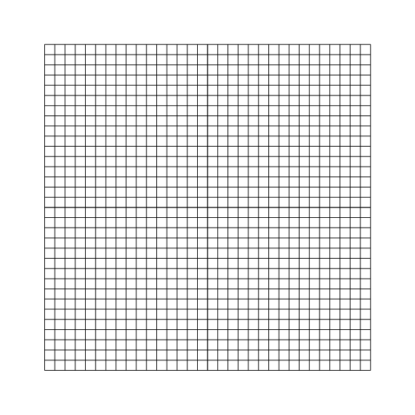
Mesh for l=5
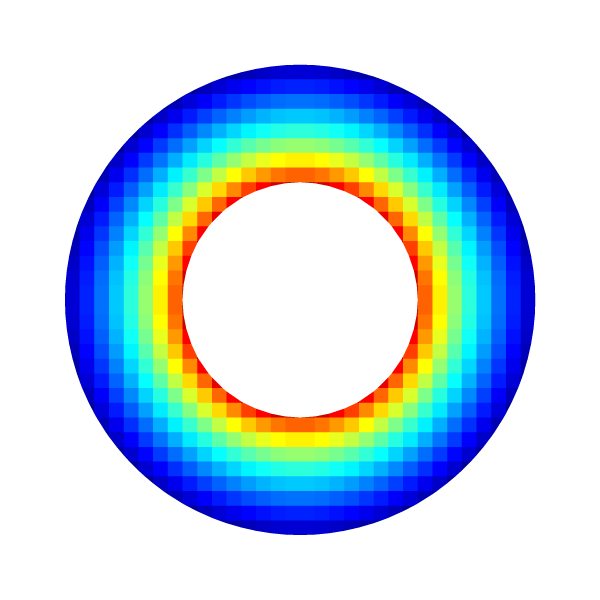
Angular velocity for l=5

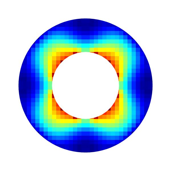
Pressure field for l=5
Error field for l=5
Velocity profile
reset
set terminal svg font ",16"
set key top right spacing 1.1
set grid
set xlabel 'r'
set ylabel 'u_theta'
set xrange [0.2:0.55]
set yrange [-0.05:0.35]

powerlaw(r,N)=r*((0.5/r)**(2./N) - 1.)/((0.5/0.25)**(2./N) - 1.)

set arrow from 0.25, graph 0 to 0.25, graph 1 nohead
set arrow from 0.5, graph 0 to 0.5, graph 1 nohead
plot powerlaw(x,1.) w l lc rgb "black" t 'analytic',		\
'out' u 1:6 w p ps 0.75 lc rgb "blue" t 'Basilisk, l=5' 
Velocity profile for l=5 (script)
Errors
reset
set terminal svg font ",16"
set key bottom left spacing 1.1
set xtics 8,4,512
set grid ytics
set ytics format "%.0e" 1.e-12,100,1.e2
set xlabel 'N'
set ylabel '||error||_{1}'
set xrange [8:512]
set yrange [1.e-6:1.e-1]
set logscale
plot 'log' u 1:4 w p ps 1.25 pt 7 lc rgb "black" t 'cut-cells', \
     ''    u 1:6 w p ps 1.25 pt 5 lc rgb "blue" t 'full cells', \
     ''    u 1:2 w p ps 1.25 pt 2 lc rgb "red" t 'all cells'
Average error convergence (script)
set ylabel '||error||_{inf}'
plot '' u 1:5 w p ps 1.25 pt 7 lc rgb "black" t 'cut-cells', \
     '' u 1:7 w p ps 1.25 pt 5 lc rgb "blue" t 'full cells', \
     '' u 1:3 w p ps 1.25 pt 2 lc rgb "red" t 'all cells'
Maximum error convergence (script)
Order of convergence
We recover here the expected second-order convergence, using both a uniform and an adaptive mesh.
reset
set terminal svg font ",16"
set key bottom left spacing 1.1
set xtics 8,4,512
set ytics -4,2,4
set grid ytics
set xlabel 'N'
set ylabel 'Order of ||error||_{1}'
set xrange [8:512]
set yrange [-4:4.5]
set logscale x

# Asymptotic order of convergence

ftitle(b) = sprintf(", asymptotic order n=%4.2f", -b);
Nmin = log(128);
f1(x) = a1 + b1*x; # cut-cells
f2(x) = a2 + b2*x; # full cells
f3(x) = a3 + b3*x; # all cells

fit [Nmin:*][*:*] f1(x) '< sort -k 1,1n log | awk "!/#/{print }"' u (log($1)):(log($4)) via a1,b1; # cut-cells
fit [Nmin:*][*:*] f2(x) '< sort -k 1,1n log | awk "!/#/{print }"' u (log($1)):(log($6)) via a2,b2; # full-cells
fit [Nmin:*][*:*] f3(x) '< sort -k 1,1n log | awk "!/#/{print }"' u (log($1)):(log($2)) via a3,b3; # all cells

plot '< sort -k 1,1n log | awk "!/#/{print }" | awk -f ../data/order.awk' u 1:4 w lp ps 1.25 pt 7 lc rgb "black" t 'cut-cells'.ftitle(b1), \
     '< sort -k 1,1n log | awk "!/#/{print }" | awk -f ../data/order.awk' u 1:6 w lp ps 1.25 pt 5 lc rgb "blue" t 'full cells'.ftitle(b2), \
     '< sort -k 1,1n log | awk "!/#/{print }" | awk -f ../data/order.awk' u 1:2 w lp ps 1.25 pt 2 lc rgb "red" t 'all cells'.ftitle(b3)
Order of convergence of the average error (script)
set ylabel 'Order of ||error||_{inf}'

# Asymptotic order of convergence

fit [Nmin:*][*:*] f1(x) '< sort -k 1,1n log | awk "!/#/{print }"' u (log($1)):(log($5)) via a1,b1; # cut-cells
fit [Nmin:*][*:*] f2(x) '< sort -k 1,1n log | awk "!/#/{print }"' u (log($1)):(log($7)) via a2,b2; # full-cells
fit [Nmin:*][*:*] f3(x) '< sort -k 1,1n log | awk "!/#/{print }"' u (log($1)):(log($3)) via a3,b3; # all cells

plot '< sort -k 1,1n log | awk "!/#/{print }" | awk -f ../data/order.awk' u 1:5 w lp ps 1.25 pt 7 lc rgb "black" t 'cut-cells'.ftitle(b1), \
     '< sort -k 1,1n log | awk "!/#/{print }" | awk -f ../data/order.awk' u 1:7 w lp ps 1.25 pt 5 lc rgb "blue" t 'full cells'.ftitle(b2), \
     '< sort -k 1,1n log | awk "!/#/{print }" | awk -f ../data/order.awk' u 1:3 w lp ps 1.25 pt 2 lc rgb "red" t 'all cells'.ftitle(b3)
Order of convergence of the maximum error (script)