porous1.c

Stokes flow through a complex porous medium, randomly refined

Stokes flow through a complex porous medium, randomly refined

This is similar to porous.c but tougher since the mesh refinement is now completely arbitrary (i.e. independent from the solution). This further tests robustness of the treatment of arbitrary embedded boundaries, with arbitrary levels of refinement.

#include "grid/quadtree.h"
#include "../myembed.h"
#include "../mycentered.h"
#include "view.h"

Geometry

The porous medium is the same as in porous.c. It is defined by the union of a random collection of disks. The number of disks can be varied to vary the porosity.

void p_shape (scalar c, face vector f)
{
  int ns = 800;
  double xc[ns], yc[ns], R[ns];
  srand (0);
  for (int i = 0; i < ns; i++)
    xc[i] = 0.5*noise(), yc[i] = 0.5*noise(), R[i] = 0.01 + 0.02*fabs(noise());

Once we have defined the random centers and radii, we can compute the levelset function \phi representing the embedded boundary.

Since the medium is periodic, we need to take into account all the disk images using periodic symmetries.

  vertex scalar phi[];
  foreach_vertex() {
    phi[] = HUGE;      
    for (double xp = -L0; xp <= L0; xp += L0)
      for (double yp = -L0; yp <= L0; yp += L0)
	for (int i = 0; i < ns; i++)
	  phi[] = intersection (phi[], (sq (x + xp - xc[i]) +
					sq (y + yp - yc[i]) - sq (R[i])));
    phi[] = -phi[];
  }
  fractions (phi, c, f);
  fractions_cleanup (c, f,
		     smin = 1.e-14, cmin = 1.e-14);
}

Setup

We need a field for viscosity so that the embedded boundary metric can be taken into account.

face vector muv[];

We also define a reference velocity field.

scalar un[];

We will vary the maximum level of refinement, starting from 5.

int lmax = 5;

int main()
{

The domain is 1\times 1 and periodic.

  origin (-L0/2., -L0/2.);

  periodic (left);
  periodic (bottom);

We set the maximum timestep.

  DT = 2.e-5;

We set the tolerance of the Poisson solver. Note here that we force the Poisson solver to perform at least two cycles. This improves the convergence towards a steady solution for the velocity for high levels of refinement. We also reduce the tolerance of the viscous Poisson solver as the average value of the velocity is around 10^{-6}.

  stokes       = true;
  TOLERANCE    = 1.e-3;
  TOLERANCE_MU = 1.e-7;
  NITERMIN     = 2;

We initialize the grid.

  N = 1 << (lmax);
  init_grid (N);

  run();
}

Boundary conditions

Properties

event properties (i++)
{
  foreach_face()
    muv.x[] = fm.x[];
}

Initial conditions

event init (i = 0)
{

We set the viscosity field in the event properties.

  mu = muv;

The gravity vector is aligned with the x-direction.

  const face vector g[] = {1.,0.};
  a = g;

We use “third-order” face flux interpolation.

#if ORDER2
  for (scalar s in {u, p})
    s.third = false;
#else
  for (scalar s in {u, p})
    s.third = true;
#endif // ORDER2
  
#if TREE

When using TREE and in the presence of embedded boundaries, we should also define the gradient of u at the cell center of cut-cells.

#endif // TREE

We initialize the embedded boundary. The mesh is refined randomly along the embedded boundary.

  p_shape (cs, fs);
  refine (cs[] && cs[] < 1. &&
	  level < 6 && (int)(500.*rand()/(double)RAND_MAX) == 1.);
  p_shape (cs, fs);
  refine (cs[] && cs[] < 1. &&
	  level < 7 && (int)(400.*rand()/(double)RAND_MAX) == 1.);
  p_shape (cs, fs);
  refine (cs[] && cs[] < 1. &&
	  level < 8 && (int)(300.*rand()/(double)RAND_MAX) == 1.);    
  p_shape (cs, fs);
  refine (cs[] && cs[] < 1. &&
	  level < 9 && (int)(200.*rand()/(double)RAND_MAX) == 1.);    
  p_shape (cs, fs);
  refine (cs[] && cs[] < 1. &&
	  level < 10 && (int)(100.*rand()/(double)RAND_MAX) == 1.);    
  p_shape (cs, fs);

  FILE * fp = fopen ("inter", "w");
  output_cells (fp);
  output_facets (cs, fp, fs);
  foreach()
    fprintf (fp, "cs %g %g %g\n", x, y, cs[]);
  foreach_face()
    fprintf (fp, "fs %g %g %g\n", x, y, fs.x[]);
  fclose (fp);

We also define the volume fraction at the previous timestep csm1=cs.

  csm1 = cs;

We define the no-slip boundary conditions for the velocity.

  u.n[embed] = dirichlet (0);
  u.t[embed] = dirichlet (0);
  p[embed]   = neumann (0);

  uf.n[embed] = dirichlet (0);
  uf.t[embed] = dirichlet (0);

We finally initialize the reference velocity field.

  foreach()
    un[] = u.x[];
}

Embedded boundaries

Outputs

We check for a stationary solution.

event logfile (i++; i <= 400)
{
  double avg = normf(u.x).avg, du = change (u.x, un)/(avg + SEPS);
  fprintf (stderr, "%d %d %d %d %d %d %d %d %.3g %.3g %.3g %.3g %.3g\n",
	   lmax, i,
	   mgp.i, mgp.nrelax, mgp.minlevel,
	   mgu.i, mgu.nrelax, mgu.minlevel,
	   du, mgp.resa*dt, mgu.resa, statsf(u.x).sum, normf(p).max);
  fflush (stderr);
}

Snapshots

event snapshots (t = end)
{
  scalar nu[];
  foreach()
    nu[] = sqrt (sq(u.x[]) + sq(u.y[]));
    
  view (fov = 19.3677);
      
  draw_vof ("cs", "fs", filled = -1, fc = {1,1,1});
  squares ("nu", linear = true, spread = 8);
  save ("nu.png");
  
  draw_vof ("cs", "fs", filled = -1, fc = {1,1,1});
  squares ("p", linear = false, spread = -1);
  save ("p.png");

  draw_vof ("cs", "fs", filled = -1, fc = {1,1,1});
  squares ("level", min = 5, max = 10);
  save ("level.png");
}

Results

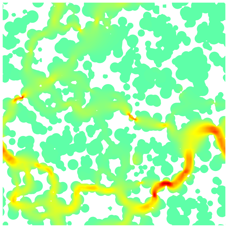
Norm of the velocity field.

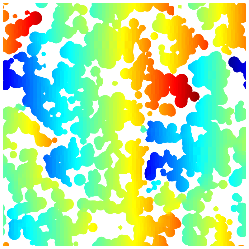
Pressure field.

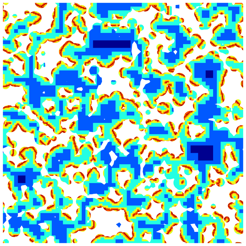
Randomly adapted mesh.

set size ratio -1
plot 'inter' w l t ''

Randomly refined mesh and embedded boundary (script)

reset
set terminal svg font ",16"
set key top spacing 1.1
set xtics -1000,100,1000
set ytics format '%.0e' 1e-18,1e-4,1e10
set xlabel 'n'
set ylabel ''
set yrange [1e-14:1e10]
set logscale y
plot 'log' u 2:9  w p pt 7  ps 0.7 lc rgb "black"     t '||u_{x}^{n+1} - u_{x}^{n}||_{inf}/||u_x^{n+1}||_1', \
     ''    u 2:10 w p pt 5  ps 0.7 lc rgb "blue"      t '||res_p||_{inf}*dt',  \
     ''    u 2:11 w p pt 2  ps 0.7 lc rgb "red"       t '||res_u||_{inf}', \
     ''    u 2:12 w p pt 12 ps 0.7 lc rgb "sea-green" t '||u_x||_{1}', \
     ''    u 2:13 w p pt 1  ps 0.7 lc rgb "coral"     t '||p||_{inf}'

Convergence history (script)