porous.c

Stokes flow through a complex porous medium

Stokes flow through a complex porous medium

The medium is periodic and described using embedded boundaries.

This tests mainly the robustness of the representation of embedded boundaries and the convergence of the viscous and Poisson solvers.

#include "grid/quadtree.h"
#include "../myembed.h"
#include "../mycentered.h"
#include "view.h"

Geometry

The porous medium is defined by the union of a random collection of disks. The number of disks can be varied to vary the porosity.

void p_shape (scalar c, face vector f)
{
  int ns = 800;
  double xc[ns], yc[ns], R[ns];
  srand (0);
  for (int i = 0; i < ns; i++)
    xc[i] = 0.5*noise(), yc[i] = 0.5*noise(), R[i] = 0.01 + 0.02*fabs(noise());

Once we have defined the random centers and radii, we can compute the levelset function $\phi$ representing the embedded boundary.

Since the medium is periodic, we need to take into account all the disk images using periodic symmetries.

  vertex scalar phi[];
  foreach_vertex() {
    phi[] = HUGE;      
    for (double xp = -L0; xp <= L0; xp += L0)
      for (double yp = -L0; yp <= L0; yp += L0)
	for (int i = 0; i < ns; i++)
	  phi[] = intersection (phi[], (sq (x + xp - xc[i]) +
					sq (y + yp - yc[i]) - sq (R[i])));
    phi[] = -phi[];
  }
  fractions (phi, c, f);
  fractions_cleanup (c, f,
		     smin = 1.e-14, cmin = 1.e-14);
}

Setup

We need a field for viscosity so that the embedded boundary metric can be taken into account.

face vector muv[];

We also define a reference velocity field.

scalar un[];

We will vary the maximum level of refinement, starting from 5.

int lmax = 5;

int main()
{

The domain is $1\times 1$ and periodic.

  size (1 [0]);
  origin (-L0/2., -L0/2.);

  periodic (left);
  periodic (bottom);

We set the maximum timestep.

  DT = 2.e-5;

We set the tolerance of the Poisson solver. Note here that we force the Poisson solver to perform at least two cycles. This improves the convergence towards a steady solution for the velocity for high levels of refinement. We also reduce the tolerance of the viscous Poisson solver as the average value of the velocity is around $10^{-6}$ .

  stokes       = true;
  TOLERANCE    = 1.e-3;
  TOLERANCE_MU = 1.e-7;
  NITERMIN     = 2;

We initialize the grid.

  N = 1 << (lmax);
  init_grid (N);

  run();
}

Boundary conditions

Properties

event properties (i++)
{
  foreach_face()
    muv.x[] = fm.x[];
}

Initial conditions

event init (i = 0)
{

We set the viscosity field in the event properties.

  mu = muv;

The gravity vector is aligned with the $x$ -direction.

  const face vector g[] = {1., 0.};
  a = g;

We use “third-order” face flux interpolation.

#if ORDER2
  for (scalar s in {u, p})
    s.third = false;
#else
  for (scalar s in {u, p})
    s.third = true;
#endif // ORDER2
  
#if TREE

When using TREE and in the presence of embedded boundaries, we should also define the gradient of u at the cell center of cut-cells.

#endif // TREE

We initialize the embedded boundary.

  p_shape (cs, fs);

We also define the volume fraction at the previous timestep csm1=cs.

  csm1 = cs;

We define the no-slip boundary conditions for the velocity.

  u.n[embed] = dirichlet (0);
  u.t[embed] = dirichlet (0);
  p[embed]   = neumann (0);

  uf.n[embed] = dirichlet (0);
  uf.t[embed] = dirichlet (0);

We finally initialize the reference velocity field.

  foreach()
    un[] = u.x[];
}

Embedded boundaries

Outputs

We check for a stationary solution.

event logfile (i++; i <= 1000)
{
  double avg = normf(u.x).avg, du = change (u.x, un)/(avg + SEPS);
  fprintf (stderr, "%d %d %d %d %d %d %d %d %.3g %.3g %.3g %.3g %.3g\n",
	   lmax, i,
	   mgp.i, mgp.nrelax, mgp.minlevel,
	   mgu.i, mgu.nrelax, mgu.minlevel,
	   du, mgp.resa*dt, mgu.resa, statsf(u.x).sum, normf(p).max);
  fflush (stderr);

If the relative change of the velocity is small enough we stop the simulation.

  if (i > 1 && (avg < 1e-9 || du < 1e-2)) {

We are interested in the permeability $k$ of the medium, which is defined by: $\displaystyle U = \frac{k}{\mu}\nabla p = \frac{k}{\mu}\rho g,$ with $U$ the average fluid velocity.

    stats s = statsf (u.x);
    fprintf (stdout, "%d %g\n", lmax, s.sum/s.volume);
    fflush (stdout);

We output fields and dump the simulation.

    char name[80];

    scalar nu[];
    foreach()
      nu[] = sqrt (sq (u.x[]) + sq (u.y[]));
    
    view (fov = 19.3677);
      
    draw_vof ("cs", "fs", filled = -1, fc = {1,1,1});
    squares ("nu", linear = false, spread = 8);
    sprintf (name, "nu-%d.png", lmax);
    save (name);
    
    draw_vof ("cs", "fs", filled = -1, fc = {1,1,1});
    squares ("p", linear = false, spread = -1);
    sprintf (name, "p-%d.png", lmax);
    save (name);

    draw_vof ("cs", "fs", filled = -1, fc = {1,1,1});
    squares ("level", min = 5, max = 10);
    sprintf (name, "level-%d.png", lmax);
    save (name);

We stop at level 10.

    if (lmax == 10)
      return 1; /* stop */

We refine the converged solution to get the initial guess for the finer level. We also reset the embedded fractions to avoid interpolation errors on the geometry.

    lmax++;
    
    adapt_wavelet ({cs,u}, (double[]){1e-2,2e-6,2e-6}, lmax);
    
    p_shape (cs, fs);

After mesh adaptation, the fluid properties need to be updated. See event adapt.

    foreach_face()
      if (uf.x[] && !fs.x[])
	uf.x[] = 0.;
    event ("properties");
  }
}

Results

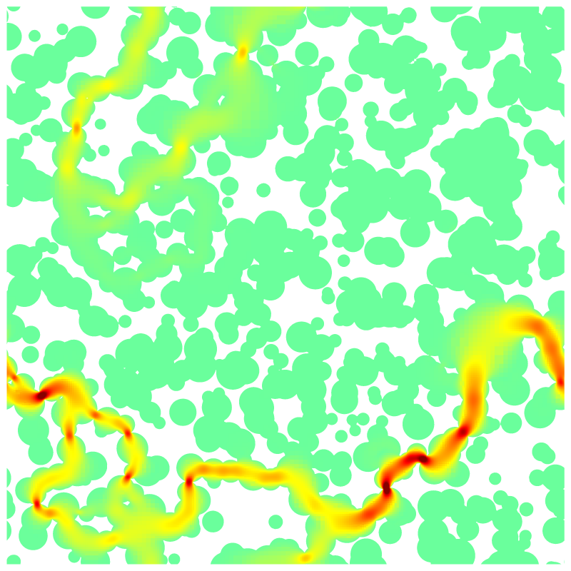
Norm of the velocity field.

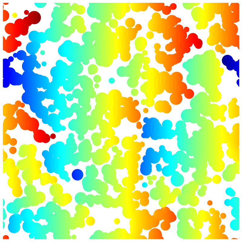
Pressure field.

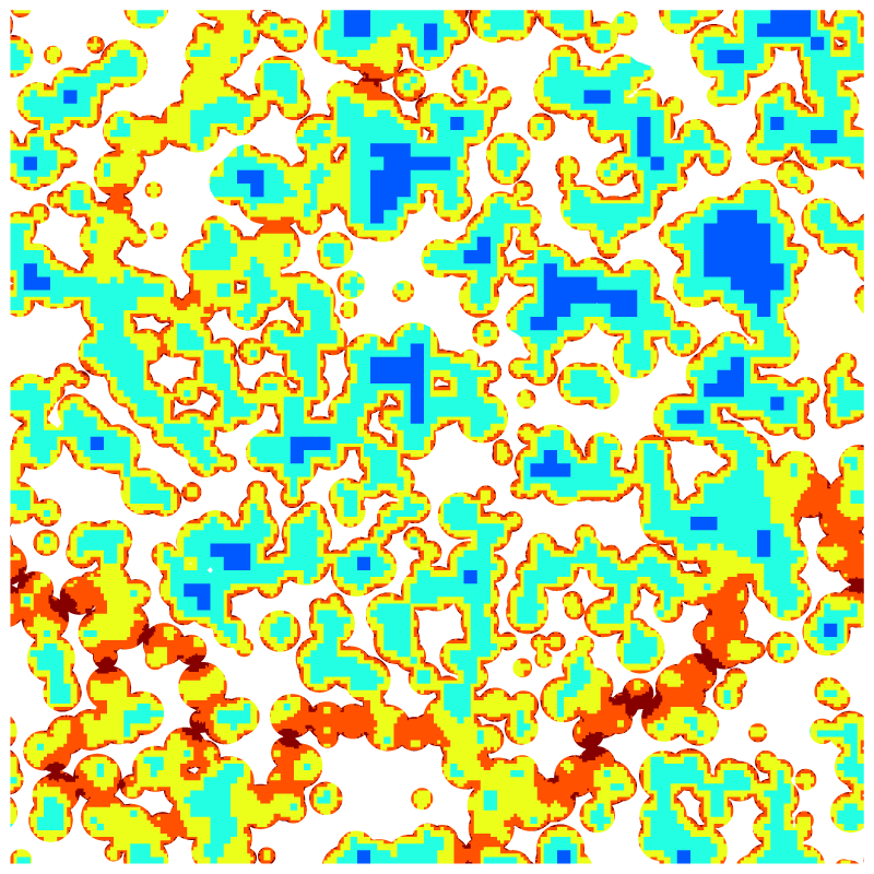
Adapted mesh, 10 levels of refinement.

Permeability as a function of resolution (script)

Convergence history (script)