sandbox/ghigo/src/test-stokes/cylinders.c

Stokes flow past a periodic array of cylinders

We compare the numerical results with the solution given by the multipole expansion of Sangani and Acrivos, 1982.

#include "grid/quadtree.h"
#include "../myembed.h"
#include "../mycentered.h"
#include "view.h"

Reference solution

This is Table 1 of Sangani and Acrivos, 1982, where the first column is the volume fraction \Phi of the cylinders and the second column is the non-dimensional drag force per unit length of cylinder F/(\mu U) with \mu the dynamic vicosity and U the average fluid velocity.

static double sangani[9][2] = {
  {0.05, 15.56},
  {0.10, 24.83},
  {0.20, 51.53},
  {0.30, 102.90},
  {0.40, 217.89},
  {0.50, 532.55},
  {0.60, 1.763e3},
  {0.70, 1.352e4},
  {0.75, 1.263e5}
};

We also define the shape of the domain. The radius of the cylinder will be computed using the volume fraction \Phi.

double radius;

void p_shape (scalar c, face vector f)
{
  vertex scalar phi[];
  foreach_vertex()
    phi[] = sq (x) + sq (y) - sq (radius);
  fractions (phi, c, f);
  fractions_cleanup (c, f,
		     smin = 1.e-14, cmin = 1.e-14);
}

Setup

We need a field for viscosity so that the embedded boundary metric can be taken into account.

face vector muv[];

We also define a reference velocity field.

scalar un[];

We vary the maximum level of refinement and the index nc of the case in the table above.

int lmax = 6, nc;

int main()
{

The domain is 1\times 1 and periodic.

  size (1 [0]);
  origin (-L0/2., -L0/2.);

  periodic (left);
  periodic (bottom);

We set the maximum timestep.

  DT = 1.e-3;

We set the tolerance of the Poisson solver. We reduce the tolerance of the viscous Poisson solver as the average value of the velocity varies between 10^{-1} and 10^{-5}, depending on the volume fraction \Phi.

  stokes       = true;
  TOLERANCE    = 1.e-4;
  TOLERANCE_MU = 1.e-8;

We run the 9 cases computed by Sangani & Acrivos. The radius is computed from the volume fraction.

  for (nc = 0; nc < 9; nc++) {
    
    radius = sqrt (sq (L0)*sangani[nc][0]/pi);

We initialize the grid.

    lmax = 6;
    N = 1 << (lmax);
    init_grid (N);

    run();
  }
}

Boundary conditions

Properties

event properties (i++)
{
  foreach_face()
    muv.x[] = fm.x[];
}

Initial conditions

event init (i = 0)
{

We set the viscosity field in the event properties.

  mu = muv;

The gravity vector is aligned with x-direction.

  const face vector g[] = {1.,0.};
  a = g;

We use “third-order” face flux interpolation.

#if ORDER2
  for (scalar s in {u, p})
    s.third = false;
#else
  for (scalar s in {u, p})
    s.third = true;
#endif // ORDER2
  
#if TREE

When using TREE and in the presence of embedded boundaries, we should also define the gradient of u at the cell center of cut-cells.

#endif // TREE

We initialize the embedded boundary.

  p_shape (cs, fs);

We also define the volume fraction at the previous timestep csm1=cs.

  csm1 = cs;

We define the no-slip boundary conditions for the velocity.

  u.n[embed] = dirichlet (0);
  u.t[embed] = dirichlet (0);
  p[embed]   = neumann (0);

  uf.n[embed] = dirichlet (0);
  uf.t[embed] = dirichlet (0);

We finally initialize the reference velocity field.

  foreach()
    un[] = u.y[];
}

Embedded boundaries

Outputs

We check for a stationary solution.

event logfile (i++; i <= 500)
{
  double avg = normf(u.x).avg, du = change (u.x, un)/(avg + SEPS);
  fprintf (stdout, "%d %d %d %d %d %d %d %d %.3g %.3g %.3g %.3g %.3g\n",
	   lmax, i,
	   mgp.i, mgp.nrelax, mgp.minlevel,
	   mgu.i, mgu.nrelax, mgu.minlevel,
	   du, mgp.resa*dt, mgu.resa, statsf(u.x).sum, normf(p).max);
  fflush (stdout);

  if (i > 1 && du < 1e-3) {

We output the non-dimensional force per unit length on the cylinder F/(\mu U), together with the corresponding value from Sangani & Acrivos and the relative error.

    coord Fp, Fmu;
    embed_force (p, u, mu, &Fp, &Fmu);
    
    stats s = statsf(u.x);
    double Phi = 1. - s.volume/sq(L0);
    double U = s.sum/s.volume;
    double F = sq(L0)/(1. - Phi);
    fprintf (stderr,
	     "%d %g %g %g %g %g %g %g\n",
	     lmax, sangani[nc][0],
	     U,
	     F/U, (Fp.x + Fmu.x)/U/sq (1 - Phi),
	     sangani[nc][1],
	     fabs(F/U - sangani[nc][1])/sangani[nc][1],
	     fabs((Fp.x + Fmu.x)/U/sq (1 - Phi) - sangani[nc][1])/sangani[nc][1]
	     ); // Why sq (1 - Phi) ??
    fflush (stderr);

We draw the mesh for one of the cases.

    if (lmax == 9 && nc == 8) {
      view (fov = 9.78488, tx = 0.250594, ty = -0.250165);
      draw_vof ("cs", "fs", lc = {1,0,0}, lw = 2);
      squares ("u.x", spread = -1);
      cells();
      save ("mesh.png");
    }

We stop at level 9.

    if (lmax == 9)
      return 1; /* stop */

We refine the converged solution to get the initial guess for the finer level. We also reset the embedded fractions to avoid interpolation errors on the geometry.

    lmax++;

    adapt_wavelet ({cs,u}, (double[]){1e-2, 2e-6, 2e-6}, lmax);
    
    p_shape (cs, fs);

After the mesh adaptation, the fluid properties need to be updated. See event adapt.

    foreach_face()
      if (uf.x[] && !fs.x[])
	uf.x[] = 0.;
    event ("properties");    
  }
}

Results

The non-dimensional drag force per unit length closely matches the results of Sangani & Acrivos. For \Phi=0.75 and level 8 there is only about 6 grid points in the width of the gap between cylinders.

set terminal svg font ",14"
set key bottom right spacing 1.1
set xlabel 'Volume fraction'
set ylabel 'k_0'
set logscale y
set grid
set key top left
plot '< grep "^8" log' u 2:6 ps 1.5 pt 7 lc rgb "black" t 'Sangani and Acrivos, 1982', \
     ''                u 2:4 ps 1.5 pt 6 lc rgb "blue"  t 'Basilisk, l=8', \
     ''                u 2:5 ps 1.5 pt 2 lc rgb "red"   t 'Basilisk, using embed{\_}force, l=8'

Non-dimensional drag force per unit length (script)

This can be further quantified by plotting the relative error. It seems that at low volume fractions, the error is independent from the mesh refinement. This may be due to other sources of errors, such as the splitting error in the projection scheme. This needs to be explored further.

set ylabel 'Relative error'
plot '< grep "^6" log' u 2:7 w lp t 'l=6', \
     '< grep "^7" log' u 2:7 w lp t 'l=7', \
     '< grep "^8" log' u 2:7 w lp t 'l=8', \
     '< grep "^9" log' u 2:7 w lp t 'l=9'

Relative error on the drag force (script)

set ylabel 'Relative error'
plot '< grep "^6" log' u 2:8 w lp t 'l=6', \
     '< grep "^7" log' u 2:8 w lp t 'l=7', \
     '< grep "^8" log' u 2:8 w lp t 'l=8', \
     '< grep "^9" log' u 2:8 w lp t 'l=9'

Relative error on the drag force computed with embed force (script)

The adaptive mesh for 9 levels of refinement illustrates the automatic refinement of the narrow gap between cylinders.

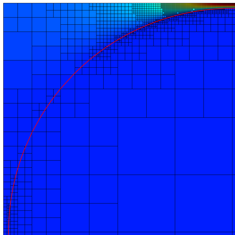
Adaptive mesh at level 9 for \Phi=0.75.

References