pipe-axi-embed.c

Developping axisymmetric pipe flow with embedded boundaries

Developping axisymmetric pipe flow with embedded boundaries

This checks that the (axisym)metric terms are properly taken into account when using embedded boundaries.

Uniform inflow u = 1 enters a pipe of radius 1 with viscosity 1/Re (Re \equiv U a/\nu, radius-based). The classical laminar entrance length (Shah & London, 1974, Durst et al. 2005) is L_{99} = 0.056 \times Re_D \times D = 0.224 \times Re \times a. With Re = 25 (default) this is 5.6\,a, comfortably inside the 8-radii-long domain.

#include "grid/multigrid.h"
#include "embed.h"
#include "axi.h"
#include "navier-stokes/centered.h"

double Re = 25.;
int LEVEL = 8;

const double LENGTH = 8. [1];    // divisible by the radius: face-aligned wall
face vector muv[];

int main (int argc, char * argv[])
{
  if (argc > 1) Re = atof (argv[1]);
  if (argc > 2) LEVEL = atoi (argv[2]);

  size (LENGTH);
  init_grid (1 << LEVEL);
  mu = muv;
  run();
}

event properties (i++) {
  const double a = 1.;
  foreach_face()
    muv.x[] = fm.x[]*a/Re;
}

Uniform inflow on the left, outflow on the right, no-slip on the wall.

u.n[left]  = dirichlet (y < 1. ? 1. : 0.);
p[left]    = neumann (0.);
pf[left]   = neumann (0.);

u.n[right] = neumann (0.);
p[right]   = dirichlet (0.);
pf[right]  = dirichlet (0.);

u.x[embed] = dirichlet (0.);
u.y[embed] = dirichlet (0.);

event init (t = 0)
{
  double eps = L0/(1 << LEVEL)/1000.;
  for (scalar s in {u, p, pf})
    s.third = true;
  solid (cs, fs, 1. - y - eps);
  fractions_cleanup (cs, fs);
  
  /* the metric updates needed to combine embed with axi */
#if AXI
  cm_update (cm, cs, fs);
  fm_update (fm, cs, fs);
  restriction ({cm, fm, cs, fs});
#endif
  
  foreach()
    u.x[] = cs[] ? (y < 1.) : 0.;
}

Diagnostics at the final time t = Re

The flow is steady well before t = Re (one radial diffusion time).

event diagnostics (t = Re)
{
  double h = L0/(1 << LEVEL);
  /* centerline profile */
  double z99 = -1.;
  for (double z = h; z < L0; z += h) {
    double uc = interpolate (u.x, z, h/4.);
    fprintf (stderr, "%g %g\n", z, uc);
    if (z99 < 0. && uc >= 0.99*2.)
      z99 = z;
  }
  fprintf (stderr,
           "# summary: Re %g LEVEL %d z99 %g u_c(exit) %g "
           "(theory: L99 = 0.224*Re = %g)\n",
           Re, LEVEL, z99, interpolate (u.x, L0 - h, h/4.), 0.224*Re);
}

Results

With the defaults (Re = 25, level 8) this gives L_{99} = 5.5625, close to the theoretical L_{99} = 5.6.

set xlabel 'z / a'
set ylabel 'u(r=0)'
set key bottom right
set arrow from 5.6, 1.0 to 5.6, 1.98 nohead dt 2 lc rgb 'blue'
set label 'L_{99} = 0.224*Re' at 5.7, 1.3 tc rgb 'blue'
set key top left
plot 'log' w l t '', \
     1.98 t '99% developed' lc rgb 'gray'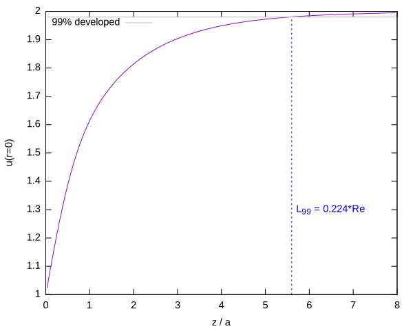

References

[durst2005]	F Durst, Subhashis Ray, Bülent Ünsal, and OA Bayoumi. The development lengths of laminar pipe and channel flows. 2005.
[shah1974]	R. K. Shah and A. L. London. Thermal boundary conditions and some solutions for laminar duct flow forced convection. Journal of Heat Transfer, 96(2):159–165, 05 1974. [ DOI \| http ]