sandbox/gally/KarmanSFD.c
SFD applied to the Kármán Vortex Street for flow around a cylinder at Re = 160
#include "embed.h"
#include "navier-stokes/centered.h"
#include "tracer.h"
We include the SFD.h module
#include "SFD.h"

scalar f[];
scalar * tracers = {f};
int maxlevel = 9;
face vector muv[];

double Reynolds = 160.;
double D = 0.125, U0 = 1.;
We set the frequency that should be kiled with the SFD method
double freq_SFD = 0.1871/0.125;The SFD will activate for a time situated between 10 and 25.
bool SFD_toggle;
event adapt_toggle (i++)
  SFD_toggle = (t >= 10. && t <= 25.);
Kármán Vortex Street
int main() {
  L0 = 8. [1];
  origin (-0.5, -L0/2.);
  N = 512;
  mu = muv;

  display_control (Reynolds, 10, 1000);
  display_control (maxlevel, 6, 12);

  run();
}

event properties (i++) {
  foreach_face()
    muv.x[] = fm.x[]*D*U0/Reynolds;
}

u.n[left]  = dirichlet(U0);
p[left]    = neumann(0.);
pf[left]   = neumann(0.);
f[left]    = dirichlet(y < 0);

u.n[right] = neumann(0.);
p[right]   = dirichlet(0.);
pf[right]  = dirichlet(0.);

u.n[embed] = dirichlet(0.);
u.t[embed] = dirichlet(0.);


event init (t = 0) {
  solid (cs, fs, sqrt(sq(x) + sq(y)) - D/2.);
  foreach()
    u.x[] = cs[] ? U0 : 0.;
}

event logfile (i++)
  fprintf (stderr, "%d %g %d %d\n", i, t, mgp.i, mgu.i);


event movies (i += 4; t <= 40.) {

  scalar omega[], m[];
  vorticity (u, omega);
  foreach() {
    m[] = cs[] - 0.5;
    if (((x < -0.4) && (y > 0.4)) && SFD_toggle)
      m[] = -0.5; // SFD on/off indicator
  }

  output_ppm (omega, file = "vort.mp4", box = {{-0.5,-0.5},{7.5,0.5}},
	      min = -10, max = 10, linear = true, mask = m);
  output_ppm (f, file = "f.mp4", box = {{-0.5,-0.5},{7.5,0.5}},
	      linear = false, min = 0, max = 1, mask = m);
}
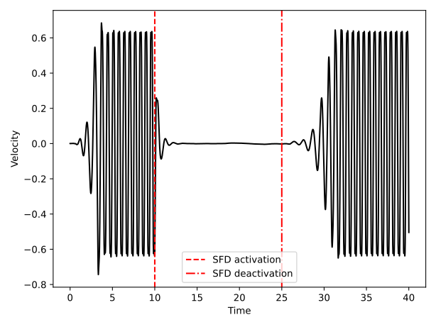
We follow the evolution of a point situated after the cylinder.
double xp, yp;

event probe (i++) {

  xp = 0.5*D + 3*D;
  yp = 0.;
  double vp = interpolate(u.y, xp, yp);

  static FILE * fp = NULL;
  if (!fp) {
    fp = fopen("probe.dat", "w");
  }
  fprintf(fp, "%g %g\n", t, vp);
}

event adapt (i++) {
  adapt_wavelet ({cs,u,f}, {1e-2,3e-2,3e-2,3e-2}, maxlevel, 4);
}
Visualisations
The SFD is activated at t = 10 and deactivated at t = 25. A dot appears on the upper-left corner when the SFD is active.
Animation of the vorticity field
Animation of the tracer field
Vertical velocity behind the cylinder through time
import numpy as np
import matplotlib.pyplot as plt

# Load data: t  vp
data = np.loadtxt("probe.dat")
t  = data[:, 0]
vp = data[:, 1]

# (De-)activation SFD
t_activation = 10
t_deactivation = 25

# Plot
plt.figure()
plt.plot(t, vp, 'k')
plt.axvline(t_activation, linestyle = '--', color = 'r', label = 'SFD activation')
plt.axvline(t_deactivation, linestyle = '-.', color = 'r', label = 'SFD deactivation')
plt.xlabel("Time")
plt.ylabel("Velocity")
#plt.xlim([0, 35])
plt.legend()
plt.tight_layout()
plt.savefig("velocity.svg")