sandbox/gally/KarmanFiltered.c
Low-pass filter
The objective of the SFD method is to drive \mathbf{q} towards the a priori unknown base state, denoted \mathbf{q_s}.
The first step consists in replacing the base state \mathbf{q_s} with a low-pass filtered version of itself, denoted \mathbf{\bar{q}}.
For practical applications, and by defining \Delta = 1/\omega_c, where \omega_c is the cutoff angular frequency of the filter, the differential form of the low-pass filter is used :
\mathbf{\dot{{\bar{q}}}} = \frac{\mathbf{q}-\mathbf{\bar{q}}}{\Delta}
The objective here is to calculate \mathbf{\bar{q}} as well as the residual \epsilon_R = ||\mathbf{q}-\mathbf{\bar{q}}||_{\mathrm{L2}} \longrightarrow 0. The solution isn’t forced to a steady state, we’re only observing the evolution of the filtered field and the residual as it is.
To calculate \mathbf{\bar{q}}, the previous equation is advanced in time using an Euler explicite scheme, and we obtain : \mathbf{\bar{q}}^{n+1}_i \simeq \left( \mathbf{q}^n_i-\mathbf{\bar{q}}^n_i \right) \frac{\delta t}{\Delta} +\mathbf{\bar{q}}^n_i
Bénard–von Kármán Vortex Street for flow around a cylinder at Re = 80
Re-use of the example code.
We use the centered Navier-Stokes solver, with embedded boundaries and advect the passive tracer f.
#include "embed.h"
#include "navier-stokes/centered.h"
#include "tracer.h"

scalar f[];
scalar * tracers = {f};
double Reynolds = 80.;
int maxlevel = 9;
face vector muv[];
We create all variables necessary for the SFD
double SFD_delta;
vector ubar[];
scalar pbar[];
double SFD_res, res;
The domain is eight units long, centered vertically.
int main() {
  L0 = 8. [1];
  origin (-0.5, -L0/2.);
  N = 512;
  mu = muv;
When using bview we can interactively control the Reynolds number and maximum level of refinement.
  display_control (Reynolds, 10, 1000);
  display_control (maxlevel, 6, 12);
We run the code for multiple different deltas.
  double SFD_deltas[] = {0.25, 6, 20};
  for (int i = 0; i < 3; i++) {
    SFD_delta = SFD_deltas[i];
    run();
  }
}
We set a constant viscosity based on the Reynolds number, the cylinder diameter D and the inflow velocity U0.
double D = 0.125, U0 = 1.;

event properties (i++) {
  foreach_face()
    muv.x[] = fm.x[]*D*U0/Reynolds;
}
The fluid is injected on the left boundary with velocity U0. The tracer is injected in the lower-half of the left boundary. An outflow condition is used on the right boundary.
u.n[left]  = dirichlet(U0);
p[left]    = neumann(0.);
pf[left]   = neumann(0.);
f[left]    = dirichlet(y < 0);

u.n[right] = neumann(0.);
p[right]   = dirichlet(0.);
pf[right]  = dirichlet(0.);
The cylinder is no-slip.
u.n[embed] = dirichlet(0.);
u.t[embed] = dirichlet(0.);

event init (t = 0) {

  solid (cs, fs, sqrt(sq(x) + sq(y)) - D/2.);
We initialize the filtered fields to the same values as the fluid properties fields.
  foreach() {
    u.x[] = cs[] ? U0 : 0.;
    ubar.x[] = cs[] ? U0 : 0.;
    ubar.y[] = 0.;
    pbar[] = 0.;
  }
}
We calculate the filtered fields at every iteration.
event bar (i++; t <= 35) {

  SFD_res = 0.;

  foreach() {

    res = sqrt( sq((u.x[] - ubar.x[])/U0) + sq((u.y[] - ubar.y[])/U0) + sq((p[] - pbar[])/sq(U0)) );
    if (res > SFD_res)
      SFD_res = res;

    ubar.x[] = (u.x[] - ubar.x[]) * (dt/SFD_delta) + ubar.x[];
    ubar.y[] = (u.y[] - ubar.y[]) * (dt/SFD_delta) + ubar.y[];
    pbar[] = (p[] - pbar[]) * (dt/SFD_delta) + pbar[];
  }

  static FILE * fbar = NULL;
  if (!fbar) {
    char filename[25];
    snprintf(filename, sizeof(filename), "res_D%.2f.dat", SFD_delta);
    fbar = fopen(filename, "w");
  }
  fprintf(fbar, "%g %g\n", t, SFD_res);
}
We check the number of iterations of the Poisson and viscous problems.
event logfile (i++)
  fprintf (stderr, "%d %g %d %d\n", i, t, mgp.i, mgu.i);
We produce animations of the vorticity fields…
event movies (i += 4; t <= 35.) {
  scalar omega[], omegabar[],  m[];
  vorticity (u, omega);
  vorticity (ubar, omegabar);

  foreach()
    m[] = cs[] - 0.5;

  char name_video[30];
  char name_videobar[30];

  snprintf(name_video, sizeof(name_video),
	   "vort_D%.2f.mp4", SFD_delta);

  snprintf(name_videobar, sizeof(name_videobar),
	   "vortbar_D%.2f.mp4", SFD_delta);

  output_ppm (omega, file = name_video, box = {{-0.5,-0.5},{7.5,0.5}},
	      min = -10, max = 10, linear = true, mask = m);
  output_ppm (omegabar, file = name_videobar, box = {{-0.5,-0.5},{7.5,0.5}},
	      min = -10, max = 10, linear = true, mask = m);
}
We adapt according to the error on the embedded geometry, velocity and tracer fields.
Residual evolution
import numpy as np
import matplotlib.pyplot as plt

# Define values
Re = 80
delta = ["0.25", "6.00", "20.00"]

# Define problem data
D = 0.125
U0 = 1
time_char = D / U0

fig, ax1 = plt.subplots(1, 3, sharey=True, figsize=(10, 3))
ax1[0].set_ylabel("Residual")

for i in range(len(delta)):

    # Load data: t  vp
    data = np.loadtxt(f"res_D{delta[i]}.dat")
    t  = data[:, 0] / time_char
    res = data[:, 1]

    # Plot
    ax1[i].plot(t, res)
    ax1[i].set_title(f"Delta = {delta[i]}")
    ax1[i].set_xlim(-0.2, 200)
    ax1[i].set_ylim(-0.2, 3)
    ax1[i].set_xlabel("Time")

plt.tight_layout()
plt.savefig("residual.png")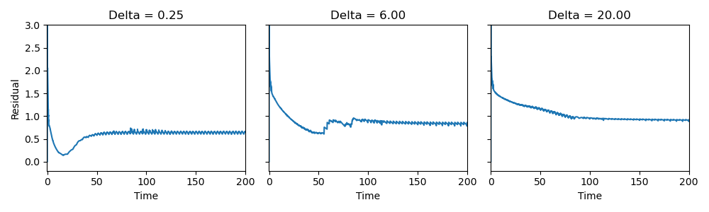
Visualisation of the vorticity fields
Animation of the unfiltered vorticity field
Unfiltered vorticity field
Animations of the filtered vorticity fields
\Delta = 0.25
\Delta = 6
\Delta = 20