global-tides.c

Global Tides
Setup
References

Global Tides

Tides are the results of the complex response of the ocean surface to the relatively simple astronomical forcing due to the variable attraction of the Moon and Sun, as illustrated in the movie below.

Top: Equilibrium astronomical tide, Bottom: Tidal response

In this example, we use the multilayer solver to simulate this response and use harmonic analysis to extract the corresponding tidal components as illustrated below.

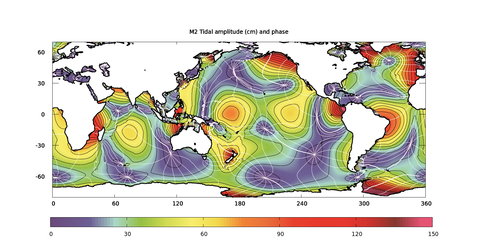
(script)

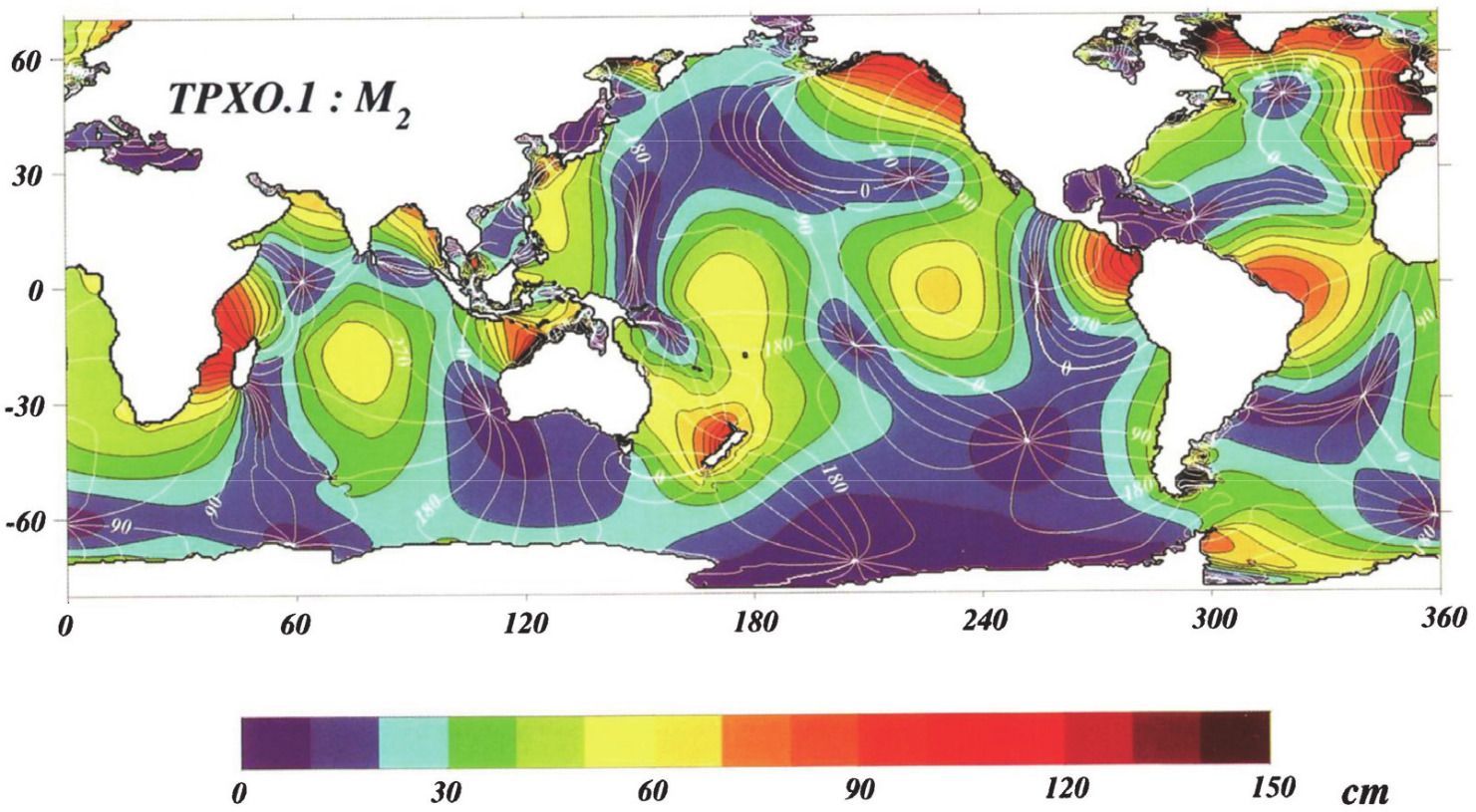
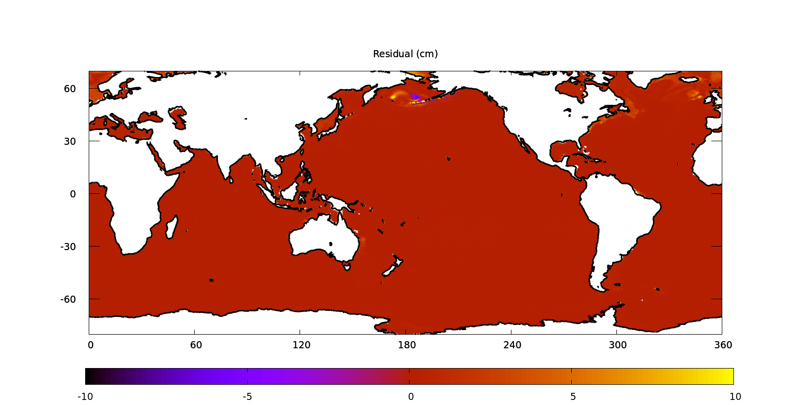
M2 component obtained by Egbert et al, 1994, plate 3, using a global inverse model and the Topex/Poseidon altimetric observations

(script)

Setup

We use the hydrostatic solver with time-implicit integration of the barotropic mode, on a regular Cartesian grid and in spherical coordinates.

#include "grid/multigrid.h"
#include "spherical.h"
#include "layered/hydro.h"
#include "layered/implicit.h"
#include "equilibrium_tide.h"

Coriolis acceleration and bottom friction

The Coriolis acceleration takes its standard definition.

const double Omega = 7.292205e-5;
#define F0() (2.*Omega*sin(y*pi/180.))

The quadratic bottom friction coefficient is set to 2 x 10^-3. The friction is only applied in the deepest wet layer.

const double Cb = 2e-3;
#define K0() (point.l > 0 && h[0,0,-1] > 10. ? 0. : h[] < dry ? HUGE : Cb*norm(u)/h[])
#include "layered/coriolis.h"

#define NL 1

Various utilities

#include "terrain.h" // for bathymetry
#include "layered/perfs.h"

const double hour = 3600., day = 86400., month = 30.*day, year = 365.*day;

The SAL correction coefficient.

const double BetaSAL = 0.1121;

We start the harmonic analysis after a spinup time of eight days.

double tspinup = 8*day;

main()

The simulation can be run in serial/OpenMP or with MPI and with a multiple of 2ⁱ⁺¹ processes. This can be done using the Makefile with e.g.:

CC='mpicc -D_MPI=8' make global-tides.tst

Command-line parameters can be passed to the code to change the spatial resolution and/or the timestep.

int main (int argc, char * argv[])
{

On a spherical grid, the sizes are given in degrees (of longitude).

  dimensions (2, 1);
  size (360);
  periodic (right);

The Earth radius, here in meters, sets the length unit.

  Radius = 6371220.;

The longitude and latitude of the lower-left corner.

  origin (0, -90);

The acceleration of gravity sets the time unit (seconds here). The standard gravity is weighted by a coefficient corresponding to the scalar approximation for “Self-Attraction and Loading” (SAL), see e.g. eq (9) and (10) in Arbic et al, 2018 and the associated discussion.

  G = 9.8*(1. - BetaSAL);

The default resolution is 1024 (longitude) x 512 (latitude) i.e. 180/512 $\approx$ 1/3 of a degree.

  if (argc > 1)
    N = atoi(argv[1]);
  else
    N = 1024;

  DT = 600;
  if (argc > 2)
    DT = atof(argv[2]);

  if (argc > 3)
    tspinup = atof(argv[3]);

A tolerance of 1 mm on the implicit solver for the free-surface height seems to be sufficient. The $\theta$ coefficient for the implicit scheme is increased slightly to add some damping to the barotropic mode (this may not be necessary).

  nl = NL;
  TOLERANCE = 1e-3;  
  theta_H = 0.55;

  run();

  system ("ffmpeg -y -i eta.mp4 eta-%04d.png;"
	  "ffmpeg -y -i tide.mp4 tide-%04d.png;"
	  "for f in eta-*.png; do"
	  "  f1=`echo $f | sed 's/eta//'`;"
	  "  montage -tile 1x2 -geometry 1024x456+0+5 tide$f1 eta$f1 montage$f1;"
	  "done;"
	  "ffmpeg -y -i montage-%04d.png -crf 18 -pix_fmt yuv420p -movflags +faststart montage.mp4;"
	  "rm -f eta-*.png tide-*.png montage-*.png;");
}

scalar zbs[], tide[];

event init (i = 0)
{

We define the equilibrium tide constituents at the start of the run.

  equilibrium_tide_constituents();

We have the option to restart (from a previous “dump” file, see below) or start from initial conditions (i.e. a “flat” ocean at rest).

  if (restore ("restart"))
    event ("metric");
  else {

The terrain uses the ETOPO2 bathymetric KDT database, which needs to be generated first. See the xyz2kdt manual for instructions.

    terrain (zbs, "~/terrain/etopo2", NULL);

We initialize the free-surface with the “equilibrium tide”, taking the SAL correction into account. We also limit the domain to $\pm 80$ degrees of latitude to avoid trouble at the poles.

    equilibrium_tide (tide, 0);
    foreach() {
      zb[] = y < -80 || y > 80 || zbs[] > - 10 ? 100 : zbs[];
      h[] = max(tide[]/(1. - BetaSAL) - zb[], 0.);
    }
  }

Boundary conditions

We set a dry, high terrain on all the “wet” domain boundaries.

  u.t[top] = dirichlet(0);
  u.t[bottom] = dirichlet(0);
  zb[top] = 1000;
  zb[bottom] = 1000;
  h[top] = 0;
  h[bottom] = 0;
}

Astronomical forcing

The astronomical forcing is added as the acceleration $g\nabla\eta_\text{eq}/(1 - \beta_\text{SAL})$ where $\eta_\text{eq}$ is the “equilibrium tide” i.e. the height the free-surface would have if the water surface equilibrated instantly with the astronomical variations of gravity.

event acceleration (i++)
{
  equilibrium_tide (tide, t);
  foreach_face() {
    double ax = G/(1. - BetaSAL)*gmetric(0)*(tide[-1] - tide[])/Delta;
    foreach_layer()
      ha.x[] -= hf.x[]*ax;
  }
}

Harmonic decomposition

We perform a harmonic decomposition of the free-surface height, using all the frequencies defined in equilibrium_tide.h.

#include "harmonic.h"

scalar etaE[];

event harmonic (t = tspinup; i++)
{
  harmonic_decomposition (eta, t, (double[]){
      Etide.Q1.omega,
      Etide.O1.omega,
      Etide.K1.omega,
      Etide.N2.omega,
      Etide.M2.omega,
      Etide.S2.omega,
      Etide.K2.omega,
      0
    }, etaE);
}

Horizontal viscosity

We add a (small) Laplacian horizontal viscosity in each layer. It is not clear whether this is really necessary i.e. how sensitive the results are to this parameter.

double nu_H = 10; // m^2/s

event viscous_term (i++)
{
  if (nu_H > 0.) {
    vector d2u[];
    foreach_layer() {
      double dry = 1.;
      foreach()
	foreach_dimension()
	d2u.x[] = 2.*(sq(fm.x[1])/(cm[1] + cm[])*u.x[1]*(h[1] > dry) +
		      sq(fm.x[])/(cm[-1] + cm[])*u.x[-1]*(h[-1] > dry) +
		      sq(fm.y[0,1])/(cm[0,1] + cm[])*u.x[0,1]*(h[0,1] > dry) +
		      sq(fm.y[0,-1])/(cm[0,-1] + cm[])*u.x[0,-1]*(h[0,-1] > dry))
	/(sq(Delta)*cm[]);
      foreach()
	foreach_dimension() {
	double n = 2.*(sq(fm.x[1])/(cm[1] + cm[])*(1. + (h[1] <= dry)) +
		       sq(fm.x[])/(cm[-1] + cm[])*(1. + (h[-1] <= dry)) +
		       sq(fm.y[0,1])/(cm[0,1] + cm[])*(1. + (h[0,1] <= dry)) +
		       sq(fm.y[0,-1])/(cm[0,-1] + cm[])*(1. + (h[0,-1] <= dry)))
	  /(sq(Delta)*cm[]);
	u.x[] = (u.x[] + dt*nu_H*d2u.x[])/(1. + dt*nu_H*n);
      }
    }
  }
}

Hourly outputs

We compute the kinetic energy in the top and bottom layer.

event outputs (t += hour)
{
  double ke = 0., keb = 0., vol = 0., volb = 0.;
  scalar etad[], nu[];
  foreach(reduction(+:ke) reduction(+:vol) reduction(+:keb) reduction(+:volb)) {
    point.l = 0;
    keb += dv()*h[]*(sq(u.x[]) + sq(u.y[]));
    volb += dv()*h[];
    foreach_layer() {
      ke += dv()*h[]*(sq(u.x[]) + sq(u.y[]));
      vol += dv()*h[];
    }
    point.l = nl - 1;
    etad[] = h[] > dry ? eta[] : 0.;
    nu[] = h[] > dry ? norm(u) : 0.;
  }

Various diagnostics.

  if (i == 0) {
    fprintf (stderr, "t ke/vol keb/vol dt "
	     "mgH.i mgH.nrelax etad.stddev nu.stddev");
    for (int l = 0; l < nl; l++)
      fprintf (stderr, " d%s%d.sum/dt", h.name, l);
    fputc ('\n', stderr);
  }
  fprintf (stderr, "%g %g %g %g %d %d %g %g", t/day, ke/vol/2., keb/volb/2., dt,
	   mgH.i, mgH.nrelax,
	   statsf (etad).stddev, statsf(nu).stddev);

This computes the rate of variation of the volume of each layer. This should be close to zero.

  static double s0[NL], t0 = 0.;
  foreach_layer() {
    double s = statsf(h).sum;
    if (i == 0)
      fprintf (stderr, " 0");
    else
      fprintf (stderr, " %g", (s - s0[_layer])/(t - t0));
    s0[_layer] = s;
  }
  fputc ('\n', stderr);
  t0 = t;
}

Movies

We make movies of the tide and of the corresponding astronomical forcing.

event movies (t = 20*day; t <= 24*day; t += 600)
{
  scalar etad[], m[];
  foreach() {
    point.l = nl - 1;
    etad[] = h[] > dry ? eta[] : 0.;
    m[] = etad[] - zbs[];
  }

Animations of the free-surface height and equilibrium tide.

  output_ppm (etad, mask = m, file = "eta.mp4", n = clamp(N,1024,2048),
	      min = -2, max = 2,
	      box = {{X0,-80},{X0+L0,80}},
	      map = jet);
  output_ppm (tide, mask = m, file = "tide.mp4", n = clamp(N,1024,2048),
	      min = -0.4, max = 0.4,
	      box = {{X0,-80},{X0+L0,80}},
	      map = jet);
}

Tide gauges

We define a list of file names, locations and descriptions and use the output_gauges() function to output timeseries (for each timestep) of $\eta$ for each location.

Gauge gauges[] = {
  // file      longitude   latitude    description
  {"dahouet", -2.25 + 360., 49.25, "Dahouët, Bretagne"},
  {NULL}
};

event gauges1 (t = tspinup; i++) {
  scalar Q1a = eta.harmonic.A[0], Q1b = eta.harmonic.B[0];
  scalar O1a = eta.harmonic.A[1], O1b = eta.harmonic.B[1];
  scalar K1a = eta.harmonic.A[2], K1b = eta.harmonic.B[2];
  scalar N2a = eta.harmonic.A[3], N2b = eta.harmonic.B[3];
  scalar M2a = eta.harmonic.A[4], M2b = eta.harmonic.B[4];
  scalar S2a = eta.harmonic.A[5], S2b = eta.harmonic.B[5];
  scalar K2a = eta.harmonic.A[6], K2b = eta.harmonic.B[6];
  scalar Z = eta.harmonic.Z;
  output_gauges (gauges, {eta, Z, etaE,
			  Q1a, Q1b, O1a, O1b, K1a, K1b, N2a, N2b, M2a, M2b, S2a, S2b, K2a, K2b});
}

Tide at Dahouët (script)

Tide at Dahouët: convergence of tidal coefficients (script)

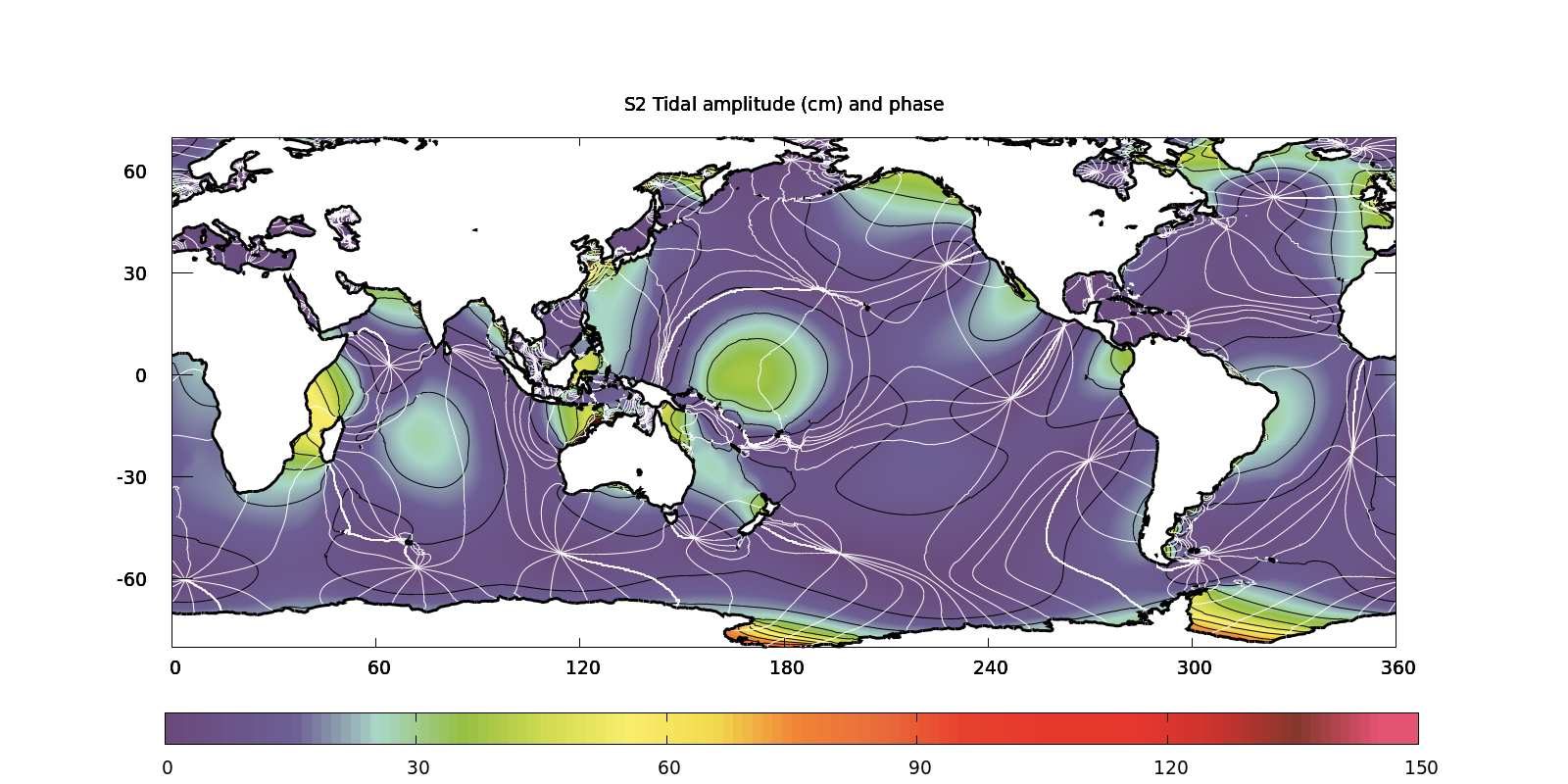
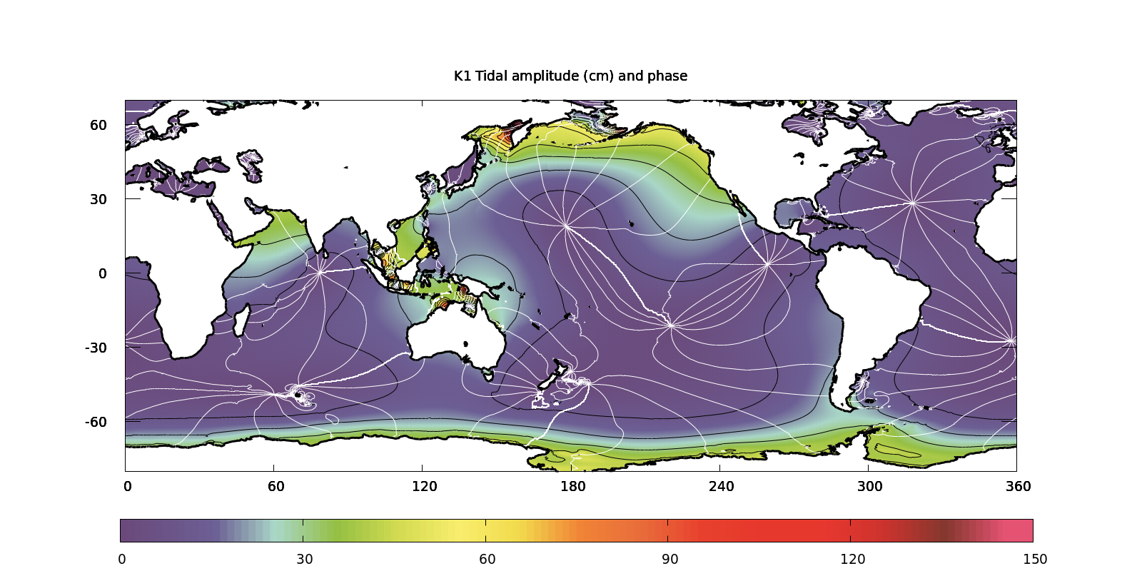
We make movies of the convergence of the harmonic decomposition into M2, S2 and K1 components.

Convergence with time of the M2 component

Convergence with time of the S2 component

Convergence with time of the K1 component

event harmonic_outputs (t = tspinup; t += hour)
{
  if (eta.harmonic.invertible) {
    scalar K1a = eta.harmonic.A[2], K1b = eta.harmonic.B[2];
    scalar M2a = eta.harmonic.A[4], M2b = eta.harmonic.B[4];
    scalar S2a = eta.harmonic.A[5], S2b = eta.harmonic.B[5];
    scalar K1[], M2[], S2[], m[];
    foreach() {
      point.l = nl - 1;
      K1[] = pow(sq(K1a[]) + sq(K1b[]), 1./4.);
      M2[] = pow(sq(M2a[]) + sq(M2b[]), 1./4.);
      S2[] = pow(sq(S2a[]) + sq(S2b[]), 1./4.);
      m[] = (h[] > dry ? eta[] : 0.) - zbs[];
    }
    output_ppm (M2, mask = m, file = "M2.mp4", n = clamp(N,1024,2048),
		linear = false,
		min = 0, max = 1.5,
		box = {{X0,-80},{X0+L0,80}},
		map = jet);
    output_ppm (S2, mask = m, file = "S2.mp4", n = clamp(N,1024,2048),
		linear = false,
		min = 0, max = 1.5,
		box = {{X0,-80},{X0+L0,80}},
		map = jet);
    output_ppm (K1, mask = m, file = "K1.mp4", n = clamp(N,1024,2048),
		linear = false,
		min = 0, max = 1.5,
		box = {{X0,-80},{X0+L0,80}},
		map = jet);
  }
}

We stop at three months and dump all fields for post-processing.

event final (t = 3*month)
{
  output_field (all, box = {{X0,-80},{X0+L0,80}});
  dump();  
}

Run times

The simulation can/should be run on parallel machines using something like:

../qcc -source -D_MPI=1 global-tides.c
scp _global-tides.c navier.lmm.jussieu.fr:gulf-stream/
mpicc -Wall -std=c99 -D_XOPEN_SOURCE=700 -O2 _global-tides.c -o global-tides -L$HOME/lib -lkdt -lm

On 32 cores of the “navier” cluster at d’Alembert, runtimes are of the order of 1/2 hour.

More results

(script)

Todo

Spherical coordinates are not great at high latitudes. A “cubed sphere” coordinate system would be nice.
The convergence of the free-surface implicit solver is not great. This may be due to the anisotropy of spherical coordinates at high latitudes.
The Self Attraction and Loading (SAL) uses a scalar approximation, which could be improved.
This could be redone with multiple stratified isopycnal layers, as in the Gulf Stream example, to get internal waves.

References

[arbic2018]	Brian K Arbic, Matthew H Alford, Joseph K Ansong, Maarten C Buijsman, Robert B Ciotti, J Thomas Farrar, Robert W Hallberg, Christopher E Henze, Christopher N Hill, Conrad A Luecke, et al. A primer on global internal tide and internal gravity wave continuum modeling in HYCOM and MITgcm. New frontiers in operational oceanography, 2018. [ DOI ]
[egbert1994]	Gary D Egbert, Andrew F Bennett, and Michael GG Foreman. TOPEX/POSEIDON tides estimated using a global inverse model. Journal of Geophysical Research: Oceans, 99(C12):24821–24852, 1994. [ DOI ]