sandbox/ysaade/f1/f1_W09.c

Mercedes-AMG F1 W09’s aerodynamics

In this code, we will attempt to simulate the flow around Lewis Hamilton’s W09, 2018’s F1 world championship winning car. Its manufacturer is the Mercedes-AMG PETRONAS F1 team.

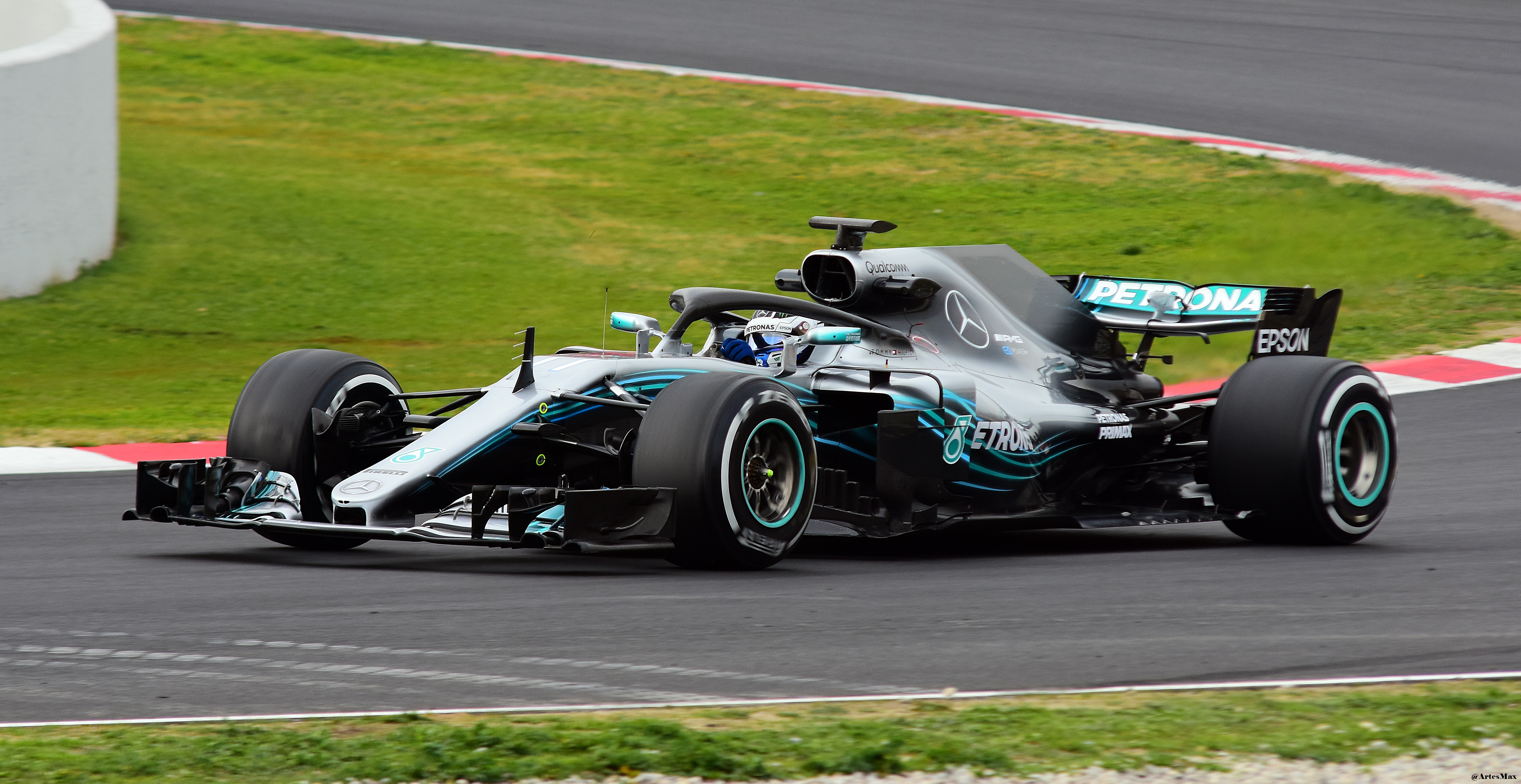
Mercedes-AMG F1 W09 EQ Power+.

To this end, we use the centered Navier-Stokes solver in a monophasic configuration.

#include "grid/octree.h"
#include "navier-stokes/centered.h"
#include "distance.h"
#include "fractions.h"
#include "lambda2.h"
#include "view.h"

Importing the geometry

We define the following scalar and face vector, which will be the vessel of the imported geometry. It is imperative that they have these names for compatibility with embed.h.

#if EMBEDDING // fixme: embedding the W09 is failing
#include "embed.h"
#else
scalar cs[];
face vector fs[];
#endif

This function computes the solid fraction given a pointer to an STL file, a tolerance (maximum relative error on distance) and a maximum level. It is implemented and already tested in many examples, such as: Distance field computation from a 3D model, Two-phase flow around RV Tangaroa, Stokes flow through a complex 3D porous medium.

void fraction_from_stl (scalar cs, face vector fs, FILE * fp,
			double eps, int maxlevel) {

We read the STL file and compute the bounding box of the model.

  coord * p = input_stl (fp);
  coord min, max;
  bounding_box (p, &min, &max);
  double maxl = -HUGE;
  foreach_dimension()
    if (max.x - min.x > maxl)
      maxl = max.x - min.x;

We initialize the distance field on the coarse initial mesh and refine it adaptively until the threshold error (on distance) is reached.

  scalar d[];
  distance (d, p);
  while (adapt_wavelet ({d}, (double[]){eps*maxl}, maxlevel).nf);

We also compute the volume fraction from the distance field. We first construct a vertex field interpolated from the centered field and then call the appropriate VOF functions.

  vertex scalar phi[];
  foreach_vertex()
    phi[] = (d[] + d[-1] + d[0,-1] + d[-1,-1] +
	     d[0,0,-1] + d[-1,0,-1] + d[0,-1,-1] + d[-1,-1,-1])/8.;

  fractions (phi, cs, fs);

This is necessary to remove degenerate fractions which could cause convergence problems if using the embedded boundary method.

#if EMBEDDING
  fractions_cleanup (cs, fs);
#endif
}

Main function

The largest dimension of the W09 is its length L\simeq 5 \ m. Although it can achieve maximum speeds a bit shy of 400\ km/h, we rein in this temple of speed to a mere U = 180 \ km/h. The resulting Reynolds number is approximately 2.5\times10^7. The computed kolmogorv scale is thus \eta=L\times Re^{-3/4}\simeq 15 \ \mu m. This DNS is therefore far from being well resolved, and is merely a proof of concept of the aerodynamics of an F1 car.

int LEVEL = 13;
double REYNOLDS = 2.5e7;

face vector muv[];

The executable takes as arguments the maximum level of refinement and the Reynolds number.

int main (int argc, char * argv[]) {
  if (argc > 1)
    LEVEL = atoi(argv[1]);
  if (argc > 2)
    REYNOLDS = atof(argv[2]);
  
  init_grid (32);

  mu = muv;

The size of the numerical domain is 4 times the length of the car. The latter is brought close to the inflow boundary so as to make room for the turbuelent wake in the numerical domain.

  size (4);
  origin (-L0/2., -3.*L0/16., 0.);

In case the geometry is not embedded, we need to tell the code that cs is a volume fraction field.

#if !EMBEDDING
  for (scalar s in {cs})
    s.refine = s.prolongation = fraction_refine;
#endif

  run();
}

Boundary conditions

If the geometry is embedded, we apply the no-slip boundary condition to the embedded surface. Otherwise, a crude method is used where we force the air velocity to be null everywhere inside the car geometry.

#if EMBEDDING
u.n[embed] = dirichlet(0.);
u.t[embed] = dirichlet(0.);
u.r[embed] = dirichlet(0.);
#else
event velocity (i++) {
  foreach()
    foreach_dimension()
      u.x[] = (1. - cs[])*u.x[];
}
#endif

The code is non dimensionlised using the car length L, its velocity U and the air density \rho. The car, cruising on a straight, is equivalent to resting still in a wind tunnel, where the air velocity is U. This is what we do in the code.

u.n[bottom] = dirichlet(1.);
p[bottom]   = neumann(0.);
pf[bottom]  = neumann(0.);
	      
u.n[top]  = neumann(0.);
p[top]    = dirichlet(0.);
pf[top]   = dirichlet(0.);

The boundary below the car is also moving at a velocity U.

u.n[back] = dirichlet(0.);
u.r[back] = dirichlet(1.);
u.t[back] = dirichlet(0.);
cs[back] = 0.;

uf.n[left] = 0.;
uf.n[right] = 0.;
uf.n[front] = 0.;

Viscosity

Viscosity is defined as the inverse of the Reynolds number.

event properties (i++) {
  foreach_face()
    muv.x[] = fm.x[]/REYNOLDS;
}

Initial conditions

The STL file of the car is read. Credit goes to a talented designer who goes by the name of TheoDev. Prior to import, the STL is scaled by L in blender so that the dimensionless length of the geometry is equal to 1. The flowing air velcoity is initialised as well.

event init (t = 0) {
  if (!restore (file = "restart")) {
    FILE * fp = fopen ("W09_scaled.stl", "r");
    fraction_from_stl (cs, fs, fp, 5e-5, LEVEL);
    fclose (fp);
  
    foreach()
      u.y[] = 1.;
  }
}

Log output

Some statistics about the simulation are outputted.

event logfile (i++)
  fprintf (stderr, "%d %g %d %d\n", i, t, mgp.i, mgu.i);

Mesh adaptation

This computation is only feasible thanks to mesh adaptation, based on both volume fraction and velocity accuracy.

event adapt (i++) {
  double uemax = 0.1;
  adapt_wavelet ({cs,u},
		 (double[]){0.01,uemax,uemax,uemax}, LEVEL, 5);
}

VOF debris

Sometimes, VOF debris appears in cells neighbouring the car which renders displaying any isosurface quite messy. A simple cleaning loop takes care of the job.

#if !EMBEDDING
event clean (i++) {
  foreach() {
    if (cs[] < 1e-6)
      cs[] = 0.;
    else if (cs[] > (1. - 1e-6))
      cs[] = 1.;
  }
}
#endif

Animation

Running with MPI-parallelism is a bit more complicated than usual since the distance() function is not parallelised yet. A reasonably simple workaround is to first generate a restart/dump file on the local machine, in a serial run, and then restore it in parallel as described here.

event dump (t = 0) {
  scalar l2[];
  lambda2 (u, l2);
  dump ("restart");
}

The simulation lasts for 1 second in physical time, during which the car travels 50 metres. PNG snapshots, out of which one can easily make a movie using ffmpeg, are saved.

event movie (t += 0.1; t <= 10) {
  scalar l2[];
  lambda2 (u, l2);
  
  char name[80];
  sprintf (name,"snapshots/snap-%g.png", t);

  clear();
  view (quat = {0.653, -0.196, -0.214, 0.699},
	fov = 30, near = 0.01, far = 1000,
	tx = 0.020, ty = -0.032, tz = -0.293,
	width = 1548, height = 936);
  box();
  double color = 0.39215686274509803;
  draw_vof (c = "cs", fc = {color,color,color},
	    lc = {color,color,color});
  squares (color = "u.y", min = -1.5, max = 1.5, linear = true);
  squares (color = "u.y", min = -1.5, max = 1.5, linear = true, n = {1,0,0});
  isosurface ("l2", -1000);
  save(name);
}