embedpotential.c

I want to share the results from Saini2022 for future references. The main finding is that the potential flow solution for bubble collapse is singular at the contact line. The potential flow solution is given by the solution of \displaystyle \boldsymbol{\nabla}^2 p = 0 is domain with BCs as shown in following figure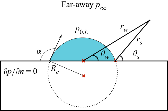 Domain and BCs for problem. Definition of different coordinate systems is also shown.

Domain and BCs for problem. Definition of different coordinate systems is also shown.

We use embed boundary to impose boundary conditions the bubble interface and solve the Laplace equation using the Poisson solver.

#include "embed.h"
#include "poisson.h"
#include "utils.h"
#include "output.h"
#include "view.h"

double R = 1;
double pinf = 10.;
scalar psi[], src[];
scalar psi1[],psi1b[];
scalar pr[];

psi[top] = dirichlet (pinf);
psi[right] = dirichlet (pinf);
psi[bottom] = neumann(0.);
psi[left] = neumann(0.);

FILE *fp,*fp2;

int main(int argc, char *argv[]){

  int maxlevel = 12;

  for(double i = 7.5; i <= 12; i+= 1.5){
    double theta0 = i*pi/18.;
    double xc = cos(theta0);

    L0 = 100.;
    size (L0);
    Y0 = 0.;
    X0 = 0.;
  
    init_grid (1 << 8);
    refine ( level <= (10 - (sqrt(x*x + y*y + z*z)/(3.) > 1)*30*pow(sqrt(x*x + y*y + z*z)/(3.) - 1.,1) ));
    refine(level < maxlevel && sqrt(sq(x - xc) + sq(y)+ z*z) > (1. - 10.*sqrt(2.)*100./(1<<12)) && sqrt(sq(x - xc) + sq(y)+ z*z) < (1. + 10.*sqrt(2.)*100./(1<<12)));
  
    vertex scalar phi[];
    foreach_vertex() {
      phi[] = sq(x - xc) + y*y - R*R;
    }
    fractions (phi, cs, fs);
    
#if TREE
    cs.refine = cs.prolongation = fraction_refine;
#endif
    restriction ({cs,fs});
    
    cm = cs;
    fm = fs;
    
    foreach (){
      src[] = 0.;
      psi[] = pinf;
    }
      
    psi[embed] = dirichlet(1.);
    
    psi.third = true;
    
    face vector alphav[];
    
    foreach_face (x) {
      alphav.x[] = y*fs.x[];
    }
    
    foreach_face (y) {
      alphav.y[] = y*fs.y[];
    }
    
    poisson (psi, src, alphav, tolerance = 1e-7, minlevel = 4);

    scalar gradpn[];

    char dpname[50];
    sprintf(dpname,"dpressure-%2.2f.dat",i);
    fp = fopen(dpname,"w");

    char dpname2[50];
    sprintf(dpname2,"dpint-%2.2f.dat",i);
    fp2 = fopen(dpname2,"w");

    foreach(){
      if (cs[] > 0. && cs[] < 1.){
	coord n = facet_normal (point, cs, fs), p;
	double alpha = plane_alpha (cs[], n);

unused variable ‘area’ [-Wunused-variable]

	double area = plane_area_center (n, alpha, &p);
	bool dirichlet;

stencils: cannot analyze point function pointers

	double vb = psi.boundary[embed] (point, point, psi, &dirichlet);
	if (dirichlet){
	  double val;
	  normalize (&n);
	  gradpn[] = dirichlet_gradient (point, psi, cs, n, p, vb, &val)/(1. - pinf);
	  fprintf(fp,"%10.9f %10.9f %10.9f\n",x,y,fabs(gradpn[]));
	  fprintf(fp2,"%10.9f %10.9f %10.9f %10.9f\n",atan2(x,y),x,y,fabs(gradpn[]));
	}
	else
	  gradpn[] = 0;
      }
      else{
	gradpn[] = cs[] >= 1. ? sqrt(sq((psi[1] - psi[-1])/2/Delta) + sq((psi[0,1] - psi[0,-1])/2/Delta))/(1. - pinf): 0.;
	if(x < 5. && y < 5.)
	  fprintf(fp,"%10.9f %10.9f %10.9f\n",x,y,fabs(gradpn[]));
      }
    }

    view(fov = 4., quat = {0,0,-cos(pi/4.),cos(pi/4.)}, width = 1980, height = 1980);
    box (notics=true);
    draw_vof (c = "cs",lw=4);
    isoline (phi = "gradpn", n = 200, min = -9, max = 10);
    mirror({0,1}) {
      box (notics=true);
      draw_vof("f",lw=4);
      isoline (phi = "gradpn", n = 200, min = -9, max = 10);
    }
    char filename[80];
    sprintf(filename,"isolines-%dpiby18.png",(int)i);
    save(filename);

We output data in a file to launch a DNS simulation from initial condition given by the potential flow solution. In case of MPI, we write the data in to seperate files that can be combined later by Bash commands for ex. cat.

    char namew[50];
#if _MPI
    sprintf(namew,"data-%2.2f-%d-%d.dat",theta0,maxlevel,pid());
#else
    sprintf(namew,"data-%2.2f.dat",theta0);
#endif
    fp = fopen(namew,"w");
    if(pid() == 0)
      fprintf(fp,"%ld ",grid->tn);
    
    foreach()
      fprintf(fp,"%d %d %d %lf ",point.level,point.i,point.j,psi[]);
    fclose(fp);
    
  }

}

reset

set style line 1 linecolor rgb '#ce2d4f' dt 1 linewidth 4 ps 1 pt 7
set style line 2 linecolor rgb '#5aae61' dt 1 linewidth 4 ps 1 pt 7
set style line 3 linecolor rgb '#2b6cbb' dt 1 linewidth 4 ps 1 pt 7
set style line 4 linecolor rgb '#000000' dt 2 linewidth 4 ps 1 pt 7

set key top right horiz font "sans-serif,16"

set lmargin 9
set bmargin 4
set tmargin 3
set rmargin 2

set xlabel "{/Symbol q}_w" font "sans-serif,16"
set ylabel "{/Symbol D} p . n_B" font "sans-serif,16"

p "dpint-7.50.dat" u 1:4 w p ls 1 t "{/Symbol a} = 75^o",\
"dpint-9.00.dat" u 1:4 w p ls 2 t "{/Symbol a} = 90^o",\
"dpint-10.50.dat" u 1:4 w p ls 3 t "{/Symbol a} = 105^o",\
"dpint-12.00.dat" u 1:4 w p ls 4 t "{/Symbol a} = 120^o"

Shapes at tend (script)


import numpy as np
import sys 
import string
import math
import glob
from pylab import *
from matplotlib.colors import LogNorm, Normalize,ListedColormap
from scipy.interpolate import griddata
from matplotlib.ticker import LogLocator

params = {
    'axes.labelsize': 14,
    'font.size': 12,
    'mathtext.fontset' : 'cm',
    'font.family' : 'sans-serif',
    'legend.fontsize': 12,
    'xtick.labelsize': 12,
    'ytick.labelsize': 12,
    'xtick.major.size' : 2.,
    'ytick.major.size' : 2.,
    'xtick.minor.size' : 1.,
    'ytick.minor.size' : 1.,
    'text.usetex': False,
#    'figure.figsize': [2.15,1.85],
    'axes.linewidth' : 0.75,
    'figure.subplot.left' : 0.1,
    'figure.subplot.bottom' : 0.18,
    'figure.subplot.right' : 0.96,
    'figure.subplot.top' : 0.98,
    'savefig.dpi' : 300,
}
rcParams.update(params)
datafiles=["dpressure-7.50.dat","dpressure-9.00.dat","dpressure-12.00.dat"]

fig, ax = plt.subplots(1, 3, figsize=(6, 2), gridspec_kw={'wspace': 0.4}, sharey=True)

i=0
for file in datafiles:
    data=np.loadtxt(file)

    x, y, f = data[:, 0], data[:, 1], data[:, 2]

    xi = np.linspace(min(x) + 0.025, max(x) - 0.025, 100)
    yi = np.linspace(min(y) + 0.025, max(y) - 0.025, 100)
    xi, yi = np.meshgrid(xi, yi)

    fii = griddata((x, y), f, (xi, yi), method='linear')
    fii = np.array(fii,dtype=np.float64)
    replacement = np.nanmin(fii)
    fi = np.where(np.isnan(fii), replacement, fii)

    # Ensure valid contour levels
    if np.min(fi) == np.max(fi):
        levels = [np.min(fi)]
    else:
        levels = np.linspace(np.min(fi), np.max(fi), 15)

    contour = ax[i].contour(yi, xi, fi, levels=levels) 
    ax[i].contour(-1.*yi, xi, fi, levels=levels)

    contour.clabel(inline=True, fontsize=3)

    ax[i].set_xlabel("r")
    ax[i].set_ylabel("z")
    ax[i].set_xlim(0.,2.5)
    ax[i].set_ylim(0,2.5)
    i=i+1

ax[0].set_title(r"$\alpha = 75^\circ$")
ax[1].set_title(r"$\alpha = 90^\circ$")
ax[2].set_title(r"$\alpha = 120^\circ$")
savefig('Contours.pdf', bbox_inches='tight', pad_inches=0.3/2.54)

Contour plots (script)