sandbox/lopez/lamb.c
Stokes flow around an sphere
The analitical solution of a viscous dominant horizontal flow of magnitude U_o around an sphere of radius a is due to Horace Lamb.
The solution can be written in terms of the stream function as:
\displaystyle \Psi (r, \theta) = \frac{U_o \sin^2 \theta}{2} \left(r^2 - \frac{3ar}{2} + \frac{a^3}{2r}\right)
where we have used polar coordinates.
The velocities are obtained simply deriving the above expressions,
\displaystyle u_r(r,\theta) = \cos \theta \left( 1 +\frac{1}{2r^3} - \frac{3}{2r} \right) \quad u_\theta(r,\theta) = -\sin \theta \left( 1 -\frac{1}{4r^3} - \frac{3}{4r} \right)
where we have made dimensionless the velocity with U_o and r with the radius a. We will use the centered Navier-Stokes solver with embedded boundaries to reproduce his result.
#include "embed.h"
#include "axi.h"
#include "navier-stokes/centered.h"
#include "view.h"
The computational domain is an square box of width W where we insert an sphere of dimensionless radius 1. We set the sphere in a very large box to minimize the influence of the location of the far field boundary (W/a \simeq 100).
#define W 100

scalar un[];
int LEVEL = 10;

int main() {
  L0=W;
  X0=-W/2;
  stokes = true;
  DT = 0.1;
  TOLERANCE_MU = 1e-5;
  run();
}
The fluid is injected on the left boundary with a velocity U_o.
u.n[left]  = dirichlet(1.);
p[left]    = dirichlet(0.);
pf[left]   = dirichlet(0.);

u.n[right] = dirichlet(1.);
p[right]   = dirichlet(0.);
pf[right]  = dirichlet(0.);

//u.t[top] = dirichlet(1.);
//p[top]   = dirichlet(0.);
//pf[top]  = dirichlet(0.);
The sphere is a non-slip surface.
u.n[embed] = dirichlet(0.);
u.t[embed] = dirichlet(0.);
Expression of the exact values of the dimensionless radial and azimuthal component of the velocity are:
double vrad(double x, double y) {
  double theta = atan2(y, x), r = sqrt(x*x + y*y);
  return cos(theta)*(1. + pow(r,-3)/2. -3/(2.*r));
}
and.
double vtheta(double x, double y) {
  double theta = atan2(y, x), r = sqrt(x*x + y*y);
  return -sin(theta)*(1. - pow(r,-3)/4. -3/(4.*r));
}

event init (t = 0)
{
Viscosity is unity.
  mu = fm;
  rho = cm;
The mesh is initially refined only around the sphere up to LEVEL. The grid is unrefined as the cells are further of the sphere.
refine ( level <= (LEVEL - sqrt(sq(x) + sq(y))/5.));The variables cs and fs characterize just the geometry of the embed solid.
  vertex scalar phi[];
  foreach_vertex()
    phi[] = sq(x) + sq(y) - sq(1.);

  fractions (phi, cs, fs);
We set the initial velocity field.
  foreach()
    u.x[] = cs[] ? 1.0 : 0.;
The variables cm and fm gathers either the metric and the embed solid factors. Therefore they must be updated right after the solid factor were updated.
We check the number of iterations of the Poisson and viscous problems and the convergence to a stationary.
event logfile (i++) {
  double du= change (u.x, un);
  if (i > 0 && du < 1e-4) {
    fprintf(stderr, "#du=%g step i=%d\n",du,i);
    return 1;
  }
}
We produce a snapshot once it is converged…
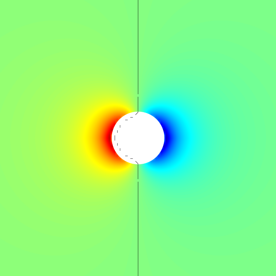
event snapshot (t = end)
{
  view (fov = 2, width = 900, height = 900);
  draw_vof ("cs", filled = -1, fc = {1,1,1} );
  squares ("u.y", spread = -1, linear = true);
  mirror ({0,1}) {
    draw_vof ("cs", filled = -1, fc = {1,1,1});
    squares ("u.x", spread = -1, linear = true);
  }
  save("veloc.png");

  clear();
  view (fov = 2, width = 900, height = 900);
  draw_vof ("cs", filled = -1, fc = {1,1,1} );
  squares ("p", spread = -1, linear = true);
  isoline ("p");
  mirror ({0,1}) {
    draw_vof ("cs", filled = -1, fc = {1,1,1});
    squares ("p", spread = -1, linear = true);
    isoline ("p");
  }
  save("press.png");

  p.nodump = pf.nodump = false;
  dump();
}

/*
When converged we plot the velocity profiles up to a distance of aprox 4
radius. */

event plotting (t = end)
{
  double alpha = 45*M_PI/180;
  double h  = 4./(99), slope = tan(alpha);
  double xo = cos(alpha);
  for (int i = 1; i <= 100; i++) {
    double x = xo + (i-1)*h, y = slope*x, r = sqrt(sq(x) + sq(y));
    double ux = interpolate (u.x, x, y); // dimensionless velocities
    double uy = interpolate (u.y, x, y);
    double vr, vt;
    vr = ux*cos(alpha) + uy*sin(alpha);
    vt =-ux*sin(alpha) + uy*cos(alpha);
    fprintf (stdout, "%g %g %g %g %g\n",
	     r, vr, vt, vrad(x,y), vtheta(x,y));
  }
}

event stop (i=500) {}
Results

Components of the velocity top: uy bottom: ux
pressure distribution around the sphere.
reset
set xlabel 'r'
set ylabel 'u_r, u_{/Symbol q}'
set arrow from 15,1 to 165,1 nohead dt 2
plot 'out' u 1:2 t 'u_r (Numerical)', \
  'out' u 1:4  w l t 'u_r (Analytical)',\
  'out' u 1:3 t 'u_{/Symbol q} (Numerical)', \
  'out' u 1:5  w l t 'u_{/Symbol q} (Analytical)'
(script)