poiseuille.c

Poiseuille flow of a Bingham fluid in a periodic channel

Poiseuille flow of a Bingham fluid in a periodic channel

We test the embedded boundaries by solving the flow of a Bingham fluid driven by gravity in a periodic channel.

#include "grid/multigrid.h"
#include "../myembed.h"
#include "../mycentered2.h"
#include "../myviscosity-viscoplastic.h"
#include "view.h"

Reference solution

#define w  (0.5) // Half-width of the channel
#define dp (1.) // Pressure gradient
#define nu (1.) // Viscosity
#define z0 (0.5) // Nondimensional length of yielded region, from 0 to 1
#define T0 ((z0)*(dp)*(w)) // Yield stress
#define uref ((T0)*(w)*sq (1 - (z0))/(2.*(nu)*(z0)))
#define tref (sq (w)/(nu))

Exact solution

We define here the exact solution for the velocity, evaluated at the center of each cell. Note that this expression is valid for the coordinate system along the direction of the channel.

static double exact (double y)
{
  return (uref)*(fabs (y/(w)) <= (z0) ? 1. :
		 1. - sq ((fabs (y/(w)) - (z0))/(1. - (z0))));
}

We also define the shape of the domain.

#define wall(y,w) ((y) - (w)) // + over, - under
#define EPS (1.e-14)

void p_shape (scalar c, face vector f)
{
  vertex scalar phi[];
  foreach_vertex() {
    phi[] = intersection (
			  -(wall (y, (w) + EPS)),
			  (wall (y, -(w) - EPS)));
  }
  boundary ({phi});
  fractions (phi, c, f);
  fractions_cleanup (c, f,
		     smin = 1.e-14, cmin = 1.e-14);
}

#if TREE

When using TREE, we try to increase the accuracy of the restriction operation in pathological cases by defining the gradient of u at the center of the cell.

void u_embed_gradient_x (Point point, scalar s, coord * g)
{  
  g->x = -y;
  g->y = 0.;
}

void u_embed_gradient_y (Point point, scalar s, coord * g)
{
  g->x = 0.;
  g->y = 0.;
}
#endif // TREE

Setup

We need a field for viscosity so that the embedded boundary metric can be taken into account. We also need a field for the density and the yield stress.

scalar rhov[];
face vector muv[], Tv[];

We also define a reference velocity field.

scalar un[];

int lvl;

int main()
{

The domain is 1\times 1 and periodic.

  L0 = 2.;
  size (L0);
  origin (-L0/2., -L0/2.);

  periodic (left);

We set the maximum timestep.

  DT = 1.e-2*(tref);

We set the tolerance of the Poisson solver.

  stokes       = true;
  TOLERANCE    = 1.e-4;
  TOLERANCE_MU = 1.e-5*(uref);

  for (lvl = 6; lvl <= 10; lvl++) {

We initialize the grid.

    N = 1 << (lvl);
    init_grid (N);

    run();
  }
}

Boundary conditions

Properties

event properties (i++)
{

We set the density and account for the metric.

  foreach()
    rhov[] = cm[];
  boundary ({rhov});

We now set the viscosity and yield stress T and account for the metric.

  foreach_face() {
    muv.x[] = (nu)*fm.x[];
    Tv.x[]  = (T0)*fm.x[];
  }
  boundary ((scalar *) {muv, Tv});
}

Initial conditions

event init (i = 0)
{

We set the viscosity and density fields in the event properties.

  rho = rhov;
  mu = muv;

We also set the yield stress and the regularization parameters.

  T = new face vector;
  Tv = T;

The gravity vector is aligned with the channel.

  const face vector g[] = {(dp), 0.};
  a = g;

We use “third-order” face flux interpolation.

#if ORDER2
  for (scalar s in {u, p})
    s.third = false;
#else
  for (scalar s in {u, p})
    s.third = true;
#endif // ORDER2
  
#if TREE

When using TREE and in the presence of embedded boundaries, we also define the gradient of u at the full cell center of cut-cells.

  foreach_dimension()
    u.x.embed_gradient = u_embed_gradient_x;
#endif // TREE

We initialize the embedded boundary.

#if TREE

When using TREE, we refine the mesh around the embedded boundary.

  astats ss;
  int ic = 0;
  do {
    ic++;
    p_shape (cs, fs);
    ss = adapt_wavelet ({cs}, (double[]) {1.e-30},
  		       maxlevel = (lvl), minlevel = (lvl) - 2);
  } while ((ss.nf || ss.nc) && ic < 100);
#endif // TREE
  
  p_shape (cs, fs);

We also define the volume fraction at the previous timestep csm1=cs.

  csm1 = cs;

We define the boundary conditions for the velocity, which is 0 on all embedded boundaries.

  u.n[embed] = dirichlet (0);
  u.t[embed] = dirichlet (0);
  p[embed]   = neumann (0);

  uf.n[embed] = dirichlet (0);
  uf.t[embed] = dirichlet (0);

We finally initialize the reference velocity field.

  foreach()
    un[] = u.x[];
}

Embedded boundaries

Outputs

event error (i++; i <= 1000)
{

We look for a stationary solution.

  double du = change (u.x, un);
  if (i > 0 && du < 1e-6)
    return 1; /* stop */
}

event logfile (t = end)
{

The total (e), partial cells (ep) and full cells (ef) errors fields and their norms are computed.

  scalar e[], ep[], ef[];
  foreach() {    
    if (cs[] == 0.)
      ep[] = ef[] = e[] = nodata;
    else {
      e[] = sqrt (sq (u.x[] - (exact (y))) +
		  sq (u.y[]));
      ep[] = cs[] < 1. ? e[] : nodata;
      ef[] = cs[] >= 1. ? e[] : nodata;
    }
  }
  norm n = normf (e), np = normf (ep), nf = normf (ef);
  
  fprintf (stderr, "%d %.3g %.3g %.3g %.3g %.3g %.3g %d %g %g %d %d %d %d\n",
	   N,
	   n.avg, n.max,
	   np.avg, np.max,
	   nf.avg, nf.max,
	   i, t, dt,
	   mgp.i, mgp.nrelax, mgu.i, mgu.nrelax);
  fflush (stderr);

  if (lvl == 6) {
    draw_vof ("cs", "fs", filled = -1, fc = {1,1,1});
    cells ();
    save ("mesh.png");

    draw_vof ("cs", "fs", filled = -1, fc = {1,1,1});
    squares ("u.x", spread = -1);
    save ("ux.png");

    draw_vof ("cs", "fs", filled = -1, fc = {1,1,1});
    squares ("u.y", spread = -1);
    save ("uy.png");

    draw_vof ("cs", "fs", filled = -1, fc = {1,1,1});
    squares ("p", spread = -1);
    save ("p.png");

    draw_vof ("cs", "fs", filled = -1, fc = {1,1,1});
    squares ("e", spread = -1);
    save ("e.png");

    yielded_region ();
    squares ("yuyz", min = 0, max = 1);
    save ("yuyz.png");
    
    foreach() {
      fprintf (stdout, "%g %g %g %g %g %g %g\n",
	       x, y,
	       u.x[]/(uref), u.y[]/(uref), p[],
	       e[], exact (y)/(uref));
      fflush (stdout);
    }
  }
}

Results

Mesh for l=6

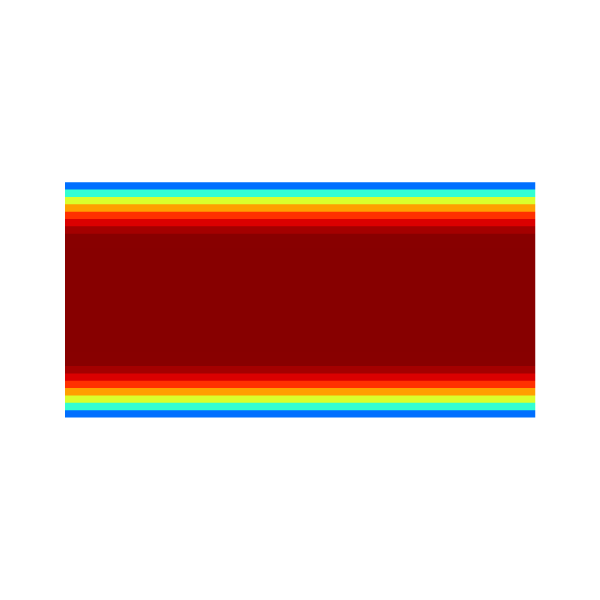
Velocity u.x for l=6

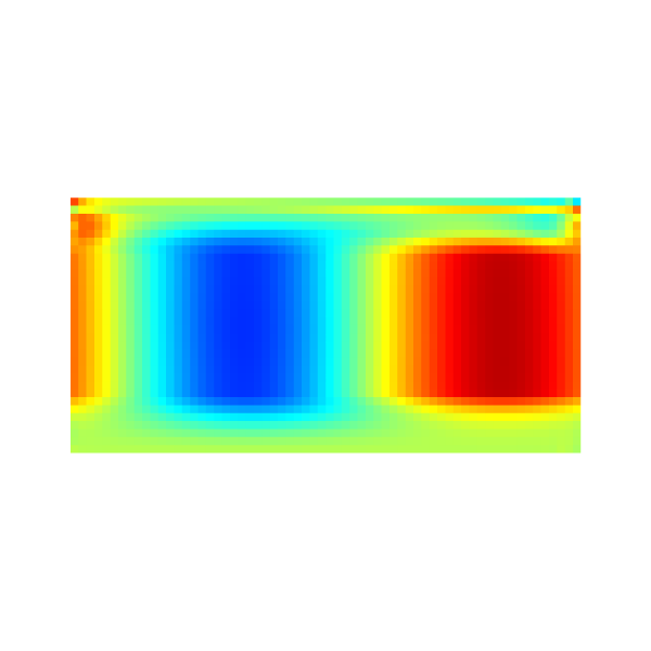
Velocity u.y for l=6

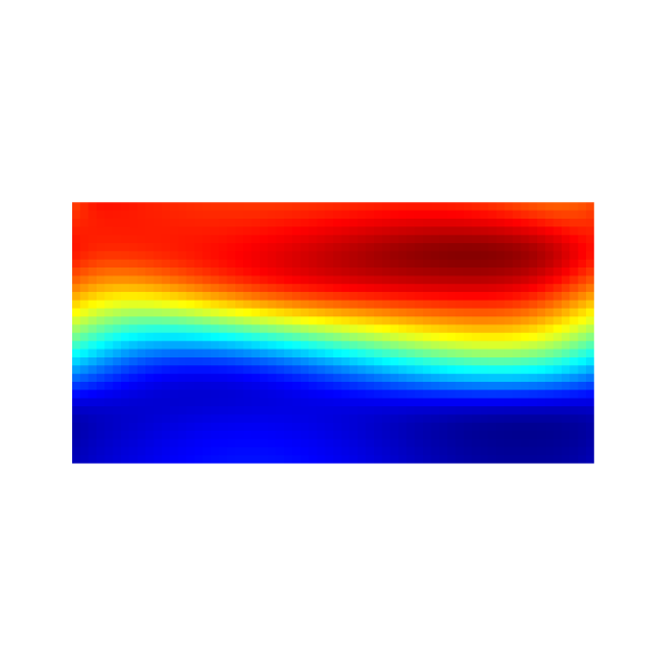
Pressure field for l=6

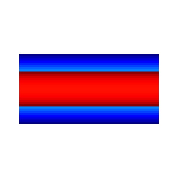
Error field for l=6

Velocity profile

reset
set terminal svg font ",16"
set key top right spacing 1.1
set xlabel 'y'
set ylabel 'u_x/u_{ref}'
set xrange [-0.5:0.5]
set yrange [-0.25:1.5]
plot 'out' u 2:7 w l lw 1.25 lc rgb "black" t "Analytic",	\
     '' u 2:3 w p ps 1.25 pt 5 lc rgb "blue" t "Basilisk"

Horizontal velocity u.x (script)

set ylabel 'err'
set yrange [0:*]
plot 'out' u 2:6 w l lw 1.25 lc rgb "black" t "Basilisk"

Error (script)

Errors

set key bottom left
set xtics 32,4,2048
set grid ytics
set ytics format "%.0e" 1.e-14,100,1.e2
set xlabel 'N'
set ylabel '||error||_{1}'
set xrange [32:2048]
set yrange [1.e-14:1.e-1]
set logscale
plot 'log' u 1:4 w p ps 1.25 pt 7 lc rgb "black" t 'cut-cells', \
     ''    u 1:6 w p ps 1.25 pt 5 lc rgb "blue" t 'full cells', \
     ''    u 1:2 w p ps 1.25 pt 2 lc rgb "red" t 'all cells'

Average error convergence (script)

set ylabel '||error||_{inf}'
plot '' u 1:5 w p ps 1.25 pt 7 lc rgb "black" t 'cut-cells', \
     '' u 1:7 w p ps 1.25 pt 5 lc rgb "blue" t 'full cells', \
     '' u 1:3 w p ps 1.25 pt 2 lc rgb "red" t 'all cells'

Maximum error convergence (script)

Order of convergence

reset
set terminal svg font ",16"
set key bottom left spacing 1.1
set xtics 32,4,2048
set ytics -4,2,4
set grid ytics
set xlabel 'N'
set ylabel 'Order of ||error||_{1}'
set xrange [32:2048]
set yrange [-4:4.5]
set logscale x

# Average order of convergence

ftitle(b) = sprintf(", avg order n=%4.2f", -b);

f1(x) = a1 + b1*x; # cut-cells
f2(x) = a2 + b2*x; # full cells
f3(x) = a3 + b3*x; # all cells

fit [*:*][*:*] f1(x) '< sort -k 1,1n log | awk "!/#/{print }"' u (log($1)):(log($4)) via a1,b1; # cut-cells 
fit [*:*][*:*] f2(x) '< sort -k 1,1n log | awk "!/#/{print }"' u (log($1)):(log($6)) via a2,b2; # full-cells
fit [*:*][*:*] f3(x) '< sort -k 1,1n log | awk "!/#/{print }"' u (log($1)):(log($2)) via a3,b3; # all cells

plot '< sort -k 1,1n log | awk "!/#/{print }" | awk -f ../data/order.awk' u 1:4 w lp ps 1.25 pt 7 lc rgb "black" t 'cut-cells'.ftitle(b1), \
     '< sort -k 1,1n log | awk "!/#/{print }" | awk -f ../data/order.awk' u 1:6 w lp ps 1.25 pt 5 lc rgb "blue" t 'full cells'.ftitle(b2), \
     '< sort -k 1,1n log | awk "!/#/{print }" | awk -f ../data/order.awk' u 1:2 w lp ps 1.25 pt 2 lc rgb "red" t 'all cells'.ftitle(b3)

Order of convergence of the average error (script)

set ylabel 'Order of ||error||_{inf}'

# Average order of convergence

fit [*:*][*:*] f1(x) '< sort -k 1,1n log | awk "!/#/{print }"' u (log($1)):(log($5)) via a1,b1; # cut-cells 
fit [*:*][*:*] f2(x) '< sort -k 1,1n log | awk "!/#/{print }"' u (log($1)):(log($7)) via a2,b2; # full-cells
fit [*:*][*:*] f3(x) '< sort -k 1,1n log | awk "!/#/{print }"' u (log($1)):(log($3)) via a3,b3; # all cells

plot '< sort -k 1,1n log | awk "!/#/{print }" | awk -f ../data/order.awk' u 1:5 w lp ps 1.25 pt 7 lc rgb "black" t 'cut-cells'.ftitle(b1), \
     '< sort -k 1,1n log | awk "!/#/{print }" | awk -f ../data/order.awk' u 1:7 w lp ps 1.25 pt 5 lc rgb "blue" t 'full cells'.ftitle(b2), \
     '< sort -k 1,1n log | awk "!/#/{print }" | awk -f ../data/order.awk' u 1:3 w lp ps 1.25 pt 2 lc rgb "red" t 'all cells'.ftitle(b3)

Order of convergence of the maximum error (script)