torque.c

Torque on a sphere in a Couette flow

Torque on a sphere in a Couette flow

We compute here the hydrodynamic torque acting on a sphere held fixed in a Couette flow with \dot{\gamma} = 1 and \mathbf{u} = \left[ \dot{\gamma}y,\, 0,\, 0 \right] and compare it to the Stokes analytical formula: \displaystyle T = 8 \pi \mu R^3 \omega, where \omega = -\dot{\gamma}/2 is the angular velocity around the sphere.

We solve here the Stokes equations and add the sphere using an embedded boundary on an adaptive grid.

#include "grid/octree.h"
#include "../myembed.h"
#include "../mycentered.h"
#include "view.h"

Reference solution

#define d       (1.)
#define uref    ((L0)/2.)
#define tref    (sq (d)/(1.)) // d^2/nu
#define Tstokes (-8.*pi*1.*cube ((d)/2)*1./2.) // Stokes torque

We also define the shape of the domain.

#define sphere(x,y,z) (sq (x) + sq (y) + sq (z) - sq ((d)/2.))

void p_shape (scalar c, face vector f)
{
  vertex scalar phi[];
  foreach_vertex()
    phi[] = (sphere (x, y, z));
  boundary ({phi});
  fractions (phi, c, f);
  fractions_cleanup (c, f,
		     smin = 1.e-14, cmin = 1.e-14);
}

Setup

We need a field for viscosity so that the embedded boundary metric can be taken into account.

face vector muv[];

We also define a reference velocity field.

scalar un[];

Finally, we define the mesh adaptation parameters.

#define lmin (6) // Min mesh refinement level (l=6 is 2pt/D)
#define lmax (9) // Max mesh refinement level (l=9 is 16pt/D)
#define cmax (1.e-2*(uref)) // Absolute refinement criteria for the velocity field

int main ()
{

The domain is 32\times 32 \times 32.

  L0 = 32.;
  size (L0);
  origin (-L0/2., -L0/2., -L0/2.);

  periodic (left);
  periodic (back);

We set the maximum timestep.

  DT = 1.e-2*(tref);

We set the tolerance of the Poisson solver.

  stokes       = true;
  TOLERANCE    = 1.e-4;
  TOLERANCE_MU = 1.e-4*(uref);

We initialize the grid.

  N = 1 << (lmin);
  init_grid (N);
  
  run();
}

Boundary conditions

We apply Couette flow boundary conditions.

u.n[bottom] = dirichlet (0);
u.t[bottom] = dirichlet (0);
u.r[bottom] = dirichlet (-(uref));
p[bottom]   = neumann (0);

u.n[top] = dirichlet (0);
u.t[top] = dirichlet (0);
u.r[top] = dirichlet ((uref));
p[top]   = neumann (0);

We give boundary conditions for the face velocity to “potentially” improve the convergence of the multigrid Poisson solver.

uf.n[bottom] = 0;
uf.n[front]  = 0;

Properties

event properties (i++)
{
  foreach_face()
    muv.x[] = fm.x[];
  boundary ((scalar *) {muv});
}

Initial conditions

event init (i = 0)
{

We set the viscosity field in the event properties.

  mu = muv;

We use “third-order” face flux interpolation.

#if ORDER2
  for (scalar s in {u, p})
    s.third = false;
#else
  for (scalar s in {u, p})
    s.third = true;
#endif // ORDER2
  
#if TREE

When using TREE and in the presence of embedded boundaries, we should also define the gradient of u at the cell center of cut-cells.

#endif // TREE

We initialize the embedded boundary.

#if TREE

When using TREE, we refine the mesh around the embedded boundary.

  astats ss;
  int ic = 0;
  do {
    ic++;
    p_shape (cs, fs);
    ss = adapt_wavelet ({cs}, (double[]) {1.e-30},
			maxlevel = (lmax), minlevel = (1));
  } while ((ss.nf || ss.nc) && ic < 100);
#endif // TREE
  
  p_shape (cs, fs);

We also define the volume fraction at the previous timestep csm1=cs.

  csm1 = cs;

We define the no-slip boundary conditions for the velocity.

  u.n[embed] = dirichlet (0);
  u.t[embed] = dirichlet (0);
  u.r[embed] = dirichlet (0);
  p[embed]   = neumann (0);

  uf.n[embed] = dirichlet (0);
  uf.t[embed] = dirichlet (0);
  uf.r[embed] = dirichlet (0);

We initialize the velocity to speed-up convergence.

  foreach()
    u.x[] = cs[]*y;
  boundary ((scalar *) {u});

We finally initialize the reference velocity field.

  foreach()
    un[] = u.x[];  
}

Embedded boundaries

#if TREE
event adapt (i++)
{
  adapt_wavelet ({cs,u}, (double[]) {1.e-2,(cmax),(cmax),(cmax)},
  		 maxlevel = (lmax), minlevel = (1));

We also reset the embedded fractions to avoid interpolation errors on the geometry.

  p_shape (cs, fs);
}
#endif // TREE

Outputs

We look for a stationary solution.

event logfile (i++; t < 10.*(tref))
{
  coord Tp, Tmu, p_p = {0, 0, 0};
  embed_torque (p, u, mu, p_p, &Tp, &Tmu);
  double dT = fabs (fabs (Tmu.z + Tp.z) - (-Tstokes))/(-Tstokes);
  fprintf (stderr, "%d %g %g %g %g %g\n",
	   i, t/(tref), dt/(tref),
	   Tp.z + Tmu.z, (Tstokes), dT);
  fflush (stderr);

  double du = change (u.x, un);
  if (i > 10 && du < 1e-6)
    return 1; /* stop */
}

event snapshot (t = end)
{
  view (fov = 20,
	tx = 0., ty = 0, bg = {1,1,1},
	width = 400, height = 400);
  squares ("u.x");
  draw_vof ("cs", "fs", lw = 1);
  save ("u.png");
}

Results

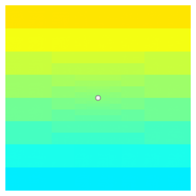
Velocity u.x

reset
set terminal svg font ",16"
set key bottom left spacing 1.1
set xtics 0,5,10
set ytics -20,2,10
set xlabel 't/(d^2/\nu)'
set ylabel 'T_z'
set xrange [1.e-12:10]
set yrange [-5:0]
plot 'log' u 2:5 w l lw 2 lc rgb 'black' t 'Stokes', \
     ''    u 2:4 w l lw 2 lc rgb 'blue' t 'Basilisk'

Time evolution of the torque T_z (script)

set key top right
set ytics 0,5,100
set yrange [0:15]
set ylabel 'err (%)'
plot 'log' u 2:(100.*$6) w l lw 2 lc rgb 'black' t 'Basilisk'

Time evolution of the relative error (script)

References

[Stokes1851]

G.G. Stokes. On the effect of the internal friction of fluids on the motion of pendulums. 1851.