spheroid-parallel-wall.c

Spheroid moving infinitely slowly parallel to a plane surface

Spheroid moving infinitely slowly parallel to a plane surface

#include "grid/octree.h"
#include "../myembed.h"
#include "../mycentered.h"
#include "../myspheroid.h"
#include "../myperfs.h"
#include "view.h"

Reference solution

#define gamma  (2.)  // Aspect ratio a/r
#define radius (0.5)
#define d      (spheroid_diameter_sphere ((radius), (gamma))) // Diameter of the sphere of equivalent volume
#define gap    (1.1) // Distance between the wall and the center of the spheroid, g/a = 1.1

We then define the incidience angle \phi (rotation along the z-axis).

#if PHI // 0, 22, 45, 66, 90
#define phi   (((double) (PHI))/180.*M_PI)
#else // phi = 0
#define phi   (0.) // incidence angle
#endif // PHI

#define nu    (1.)  // Viscosity

#define uref (1.)
#define tref (min (sq ((d)/(nu)), (gap)*(radius)*(gamma)/(uref))) // tref = delta/u

We also define the shape of the domain. Note here that p_p is the position of the center of the spheroid.

To avoid a high concentration of cells near a domain boundary (pathological case for Basilisk) and to increase the accuracy of the boundary treatment, we define the wall towards which the particle is “moving” using embedded boundaries instead of using a boundary of the domain.

#define h (-(256.)*(d)/2. + 1.1*(d) + 1.e-8) // Position of the wall
#define spheroid(x,y,z) (sq ((x)/(radius)) + sq ((y)/(radius)/(gamma)) + sq ((z)/(radius)) - 1.)
#define wall(x,w) ((x) - (w)) // + over, - under
coord p_p;

void p_shape (scalar c, face vector f, coord p)
{
  vertex scalar psi[];
  foreach_vertex() {

    // Rotated coordinates around the z-axis at the position p
    double xrot = p.x - (x - p.x)*sin (M_PI/2. - (phi)) + (y - p.y)*cos (M_PI/2. - (phi));
    double yrot = p.y + (x - p.x)*cos (M_PI/2. - (phi)) + (y - p.y)*sin (M_PI/2. - (phi));
    double zrot = z;
    
    psi[] = intersection (
    			  (spheroid ((xrot - p.x), (yrot - p.y), (zrot - p.z))),
    			  (wall ((x), (h)))
    			  );
  }
  boundary ({psi});
  fractions (psi, c, f);
  fractions_cleanup (c, f,
  		     smin = 1.e-14, cmin = 1.e-14);
}

Setup

We need a field for viscosity so that the embedded boundary metric can be taken into account.

face vector muv[];

We also define a reference velocity field.

scalar un[];

Finally, we define the mesh adaptation parameters.

#define lmem (6) // Initial mesh refinement level to avoid memory overload
#define lmin (9) // Min mesh refinement level (l=1 is 2pt/a for L0=256)
#define lmax (15) // Max mesh refinement level (l=15 is 128pt/a for L0=256)
#define cmax (1.e-3*(uref)) // Absolute refinement criteria for the velocity field
#define sphere(x,y,z,diam) (sq ((x)) + sq ((y)) + sq ((z)) - sq ((diam)/2.))
 
int main ()
{

The domain is 256\times 256 \times 256.

  L0 = 256.*(d);
  size (L0);
  origin (-(L0)/2., -(L0)/2., -(L0)/2.);

We set the maximum timestep.

  DT = 1.e-2*(tref);

We set the tolerance of the Poisson solver.

  stokes       = true;
  TOLERANCE    = 1.e-6;
  TOLERANCE_MU = 1.e-6*(uref);
  NITERMAX     = 200; // Convergence is more difficult for smaller gap sizes

We initialize the grid.

  N = 1 << (lmem);
  init_grid (N);
  
  run();
}

Boundary conditions

We impose no-slip boundary conditions on all boundaries as the fluid is supposed to be at rest at an infinite distance from the plane.

u.n[left] = dirichlet (0);
u.t[left] = dirichlet (0);
u.r[left] = dirichlet (0);
p[left]   = neumann (0);

u.n[right] = dirichlet (0);
u.t[right] = dirichlet (0);
u.r[right] = dirichlet (0);
p[right]   = neumann (0);

u.n[bottom] = dirichlet (0);
u.t[bottom] = dirichlet (0);
u.r[bottom] = dirichlet (0);
p[bottom]   = neumann (0);

u.n[top] = dirichlet (0);
u.t[top] = dirichlet (0);
u.r[top] = dirichlet (0);
p[top]   = neumann (0);

u.n[back] = dirichlet (0);
u.t[back] = dirichlet (0);
u.r[back] = dirichlet (0);
p[back]   = neumann (0);

u.n[front] = dirichlet (0);
u.t[front] = dirichlet (0);
u.r[front] = dirichlet (0);
p[front]   = neumann (0);

We give boundary conditions for the face velocity to “potentially” improve the convergence of the multigrid Poisson solver.

uf.n[left]   = 0;
uf.n[right]  = 0;
uf.n[bottom] = 0;
uf.n[top]    = 0;
uf.n[back]   = 0;
uf.n[front]  = 0;

Properties

event properties (i++)
{
  foreach_face()
    muv.x[] = (nu)*fm.x[];
  boundary ((scalar *) {muv});
}

Initial conditions

event init (i = 0)
{

We set the viscosity field in the event properties.

  mu = muv;

We use “third-order” face flux interpolation.

#if ORDER2
  for (scalar s in {u, p})
    s.third = false;
#else
  for (scalar s in {u, p})
    s.third = true;
#endif // ORDER2
  
#if TREE

When using TREE and in the presence of embedded boundaries, we should also define the gradient of u at the cell center of cut-cells.

#endif // TREE

We initialize the embedded boundary.

We first define the sphere’s position.

  p_p.x = (h) + (gap)*(radius)*(gamma);
  p_p.y = 0.;
  p_p.z = 0.;

If the simulation is not restarted, we define the initial mesh and the initial velocity.

Note here that we do not dump the pressure so the first drag computation after restart will be done using p=0.

  if (!restore (file = "restart")) {

#if TREE

Before defining the embedded boundaries, we refine the mesh up to lmin in the vicinity of the particle.

    if ((lmem) < (lmin)) {
      refine ((sphere ((x - p_p.x),
		       (y - p_p.y),
		       (z - p_p.z),
		       2.*((L0)/(1 << (lmem))))) < 0. &&
	      level < (lmin));
      p_shape (cs, fs, p_p);
    }

When using TREE, we refine the mesh around the embedded boundary.

    astats ss;
    int ic = 0;
    do {
      ic++;
      p_shape (cs, fs, p_p);
      ss = adapt_wavelet ({cs}, (double[]) {1.e-2},
			  maxlevel = (lmax), minlevel = (1));
    } while ((ss.nf || ss.nc) && ic < 100);
#endif // TREE
  }

After initialization or restart, we still need to define the face fraction fs as it is not dumped.

  p_shape (cs, fs, p_p);

Whether restarting or not, we define the volume fraction at the previous timestep csm1=cs.

  csm1 = cs;

We define the boundary condition u_{\mathrm{ref}}\mathbf{e_y} for the velocity.

  u.n[embed] = dirichlet (0);
  u.t[embed] = dirichlet (x > (h) + fabs((gap) - 1.)*(radius)*(gamma)/2. ? (uref) : 0.);
  u.r[embed] = dirichlet (0);
  p[embed]   = neumann (0);

  uf.n[embed] = dirichlet (0);
  uf.t[embed] = dirichlet (x > (h) + fabs((gap) - 1.)*(radius)*(gamma)/2. ? (uref) : 0.);
  uf.r[embed] = dirichlet (0);

We finally initialize, even when restarting, the reference velocity field.

  foreach()
    un[] = u.y[];
}

Embedded boundaries

#if TREE
event adapt (i++)
{
  adapt_wavelet ({cs,u}, (double[]) {1.e-1,(cmax),(cmax),(cmax)},
  		 maxlevel = (lmax), minlevel = (1));

We also reset the embedded fractions to avoid interpolation errors on the geometry.

  p_shape (cs, fs, p_p);
}
#endif // TREE

Restarts and dumps

Every 100 time steps, we dump the fluid data for restarting purposes. We use a relatively small time step interval as the simulations with a large value of lmax are relatively slow.

#if DUMP
event dump_data (i += 100)
{
  // Dump fluid
  dump ("dump");
}
#endif // DUMP

event dump_end (t = end)
{
  // Dump fluid
  dump ("dump-final");  
}

Profiling

#if TRACE > 1
event profiling (i += 20) {
  static FILE * fp = fopen ("profiling", "a"); // In case of restart
  trace_print (fp, 1); // Display functions taking more than 1% of runtime.
}
#endif // TRACE

Outputs

We define a color volume fraction in order to compute the force acting only on the sphere.

scalar col[];

double Km1 = 0.;

event init (i = 0)
{
  trash ({col});
  Km1 = 0.;
}

event logfile (i++; t <= 30.*(tref))
{
  double du = change (u.y, un);

We update the color volume fraction.

  vertex scalar psi[];
  foreach_vertex() {
    double xrot = p_p.x - (x - p_p.x)*sin (M_PI/2. - (phi)) + (y - p_p.y)*cos (M_PI/2. - (phi));
    double yrot = p_p.y + (x - p_p.x)*cos (M_PI/2. - (phi)) + (y - p_p.y)*sin (M_PI/2. - (phi));
    double zrot = z;
    psi[] = (spheroid ((xrot - p_p.x), (yrot - p_p.y), (zrot - p_p.z)));
  }
  boundary ({psi});
  fractions (psi, col);
  boundary ((scalar *) {col});

We compute the hydrodynamic forces acting on the sphere.

  coord Fp, Fmu;
  embed_color_force (p, u, mu, col, &Fp, &Fmu);
  
  double Kx  = fabs (Fp.x + Fmu.x)/(6.*pi*(nu)*(uref)*(d)/2.);
  double Ky  = fabs (Fp.y + Fmu.y)/(6.*pi*(nu)*(uref)*(d)/2.);
  double Kz  = fabs (Fp.z + Fmu.z)/(6.*pi*(nu)*(uref)*(d)/2.);
  double dK = fabs (Ky - Km1);
  Km1 = Ky;

We use the default log file to output the results. However, this file will be written over if the simulation is restarted.

  fprintf (stderr, "%g %d %g %g %d %d %d %d %d %d %g %g %g %g %g %g %g %g %g %g %g %g %g %g %g\n",
	   (phi),
	   i, t/(tref), dt/(tref),
	   mgp.i, mgp.nrelax, mgp.minlevel,
	   mgu.i, mgu.nrelax, mgu.minlevel,
	   mgp.resb, mgp.resa,
	   mgu.resb, mgu.resa,
	   Fp.x, Fp.y, Fp.z,
	   Fmu.x, Fmu.y, Fmu.z,
	   Kx, Ky, Kz, dK,
	   du
	   );
  fflush (stderr);
}

Snapshots

event snapshot (t += 5.*(tref))
{
  scalar n2u[];
  foreach() {
    if (cs[] <= 0.)
      n2u[] = nodata;
    else
      n2u[] = sqrt (sq (u.x[]) + sq (u.y[]) + sq (u.z[]));
  }
  boundary ({n2u});

  stats sn2u = statsf (n2u);
  stats sux  = statsf (u.x);
  stats suy  = statsf (u.y);
  
  char name2[80];

We first plot the whole domain.

  clear ();
  view (fov = 20, camera = "front",
	tx = 1.e-12, ty = 1.e-12,
	bg = {1,1,1}, width = 800, height = 800);
  
  squares ("cs", n = {0,0,1}, alpha = 1.e-12, min = 0, max = 1, map = cool_warm);
  cells (n = {0,0,1}, alpha = 1.e-12);
  sprintf (name2, "vof-t-%.0f.png", t/(tref));
  save (name2);

  squares ("col", n = {0,0,1}, alpha = 1.e-12, min = 0, max = 1, map = cool_warm);
  cells (n = {0,0,1}, alpha = 1.e-12);
  sprintf (name2, "col-t-%.0f.png", t/(tref));
  save (name2);

  squares ("n2u", n = {0,0,1}, alpha = 1.e-12, min = 0, max = sn2u.max, map = jet);
  sprintf (name2, "nu-t-%.0f.png", t/(tref));
  save (name2);

  draw_vof ("cs", "fs", lw = 5);
  squares ("u.x", n = {0,0,1}, alpha = 1.e-12, min = sux.min, max = sux.max, map = cool_warm);
  sprintf (name2, "ux-t-%.0f.png", t/(tref));
  save (name2);

  draw_vof ("cs", "fs", lw = 5);
  squares ("u.y", n = {0,0,1}, alpha = 1.e-12, min = suy.min, max = suy.max, map = cool_warm);
  sprintf (name2, "uy-t-%.0f.png", t/(tref));
  save (name2);

We plot the mesh and embedded boundaries.

  //xy

  clear ();
  view (fov = 0.2, camera = "front",
	tx = -(p_p.x)/(L0), ty = -(p_p.y)/(L0),
	bg = {1,1,1}, width = 800, height = 800);
  
  squares ("cs", n = {0,0,1}, alpha = 1.e-12, min = 0, max = 1, map = cool_warm);
  cells (n = {0,0,1}, alpha = 1.e-12);
  sprintf (name2, "vof-xy-t-%.0f.png", t/(tref));
  save (name2);

  squares ("col", n = {0,0,1}, alpha = 1.e-12, min = 0, max = 1, map = cool_warm);
  cells (n = {0,0,1}, alpha = 1.e-12);
  sprintf (name2, "col-xy-t-%.0f.png", t/(tref));
  save (name2);
  
  squares ("n2u", n = {0,0,1}, alpha = 1.e-12, min = 0, max = sn2u.max, map = jet);
  sprintf (name2, "nu-xy-t-%.0f.png", t/(tref));
  save (name2);

  draw_vof ("cs", "fs", lw = 5);
  squares ("u.x", n = {0,0,1}, alpha = 1.e-12, min = sux.min, max = sux.max, map = jet);
  sprintf (name2, "ux-xy-t-%.0f.png", t/(tref));
  save (name2);

  draw_vof ("cs", "fs", lw = 5);
  squares ("u.y", n = {0,0,1}, alpha = 1.e-12, min = suy.min, max = suy.max, map = jet);
  sprintf (name2, "uy-xy-t-%.0f.png", t/(tref));
  save (name2);

  // xz

  clear ();
  view (fov = 0.2, camera = "top",
	tx = -(p_p.x)/(L0), ty = -(p_p.z)/(L0),
	bg = {1,1,1}, width = 800, height = 800);

  squares ("cs", n = {0,1,0}, alpha = 1.e-12, min = 0, max = 1, map = cool_warm);
  cells (n = {0,1,0}, alpha = 1.e-12);
  sprintf (name2, "vof-xz-t-%.0f.png", t/(tref));
  save (name2);

  squares ("col", n = {0,1,0}, alpha = 1.e-12, min = 0, max = 1, map = cool_warm);
  cells (n = {0,1,0}, alpha = 1.e-12);
  sprintf (name2, "col-xz-t-%.0f.png", t/(tref));
  save (name2);

  squares ("n2u", n = {0,1,0}, alpha = 1.e-12, min = 0, max = sn2u.max, map = jet);
  sprintf (name2, "nu-xz-t-%.0f.png", t/(tref));
  save (name2);

  draw_vof ("cs", "fs", lw = 5);
  squares ("u.x", n = {0,1,0}, alpha = 1.e-12, min = sux.min, max = sux.max, map = jet);
  sprintf (name2, "ux-xz-t-%.0f.png", t/(tref));
  save (name2);

  draw_vof ("cs", "fs", lw = 5);
  squares ("u.y", n = {0,1,0}, alpha = 1.e-12, min = suy.min, max = suy.max, map = jet);
  sprintf (name2, "uy-xz-t-%.0f.png", t/(tref));
  save (name2);
}

Results

Results for \phi=22

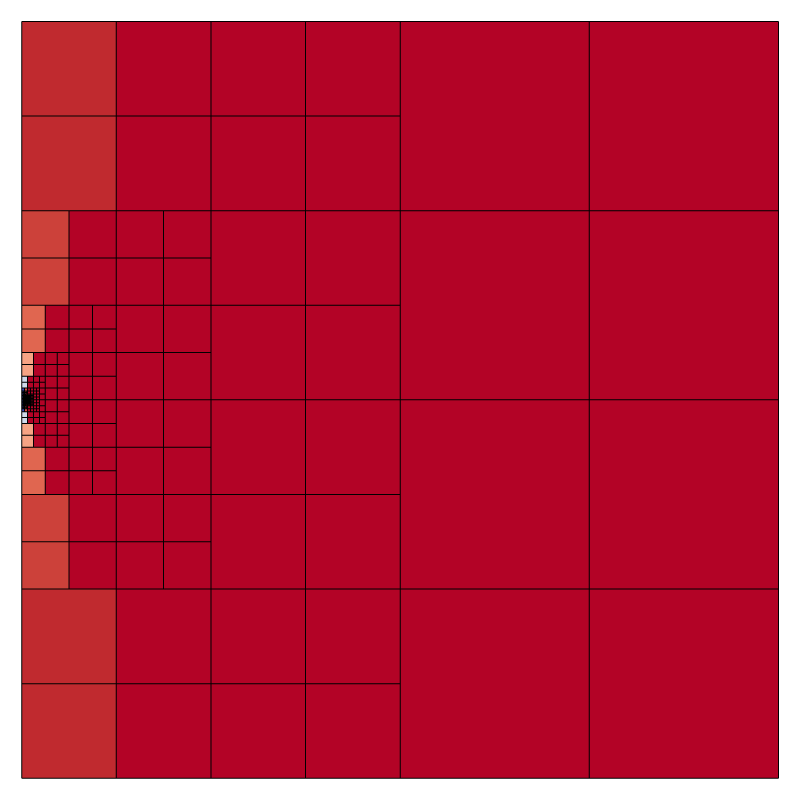
Initial mesh and embedded boundaries

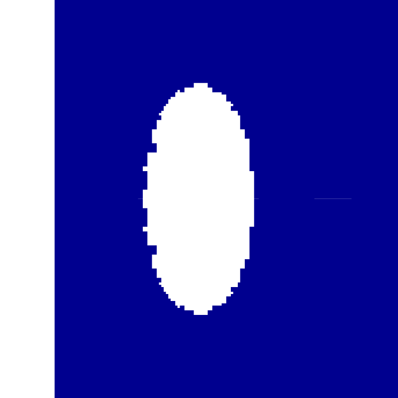
Initial velocity

reset
set terminal svg font ",16"
set key top right spacing 1.1
set grid ytics
set xtics 0,5,100
set ytics 0,0.5,10
set xlabel 't/t_{ref}'
set ylabel 'k_y'
set xrange [0:30]
set yrange [0:3]
plot 'log' u 3:22 w l lw 2 lc rgb 'blue' t 'Basilisk'

$Time evolution of the drag correction factor \kappa_y (script)$

Time evolution of the drag correction factor \kappa_y (script)

Dependence on the incidence angle \phi

set ylabel 'k_y/k_{Oberbeck}

# Aspect ratio
g = 2.;

# Oberbeck 1876
L = log ((g + sqrt (g*g - 1))/(g - sqrt (g*g - 1)))
X0 = (g*g - 1.)**(-1./2.)*L;
A0 = (g*g - 1.)**(-3./2.)*(L - 2./g*sqrt (g*g - 1.));
B0 = (g*g - 1.)**(-3./2.)*(-1./2.*L + g*sqrt (g*g - 1.));

k0  = 8./3.*g**(-1./3.)/(X0 + g*g*A0);
k90 = 8./3.*g**(-1./3.)/(X0 + B0);

f(x) = k0*cos(x/180.*pi)*cos(x/180.*pi) + k90*sin(x/180.*pi)*sin(x/180.*pi)

plot 'gamma-2/phi-0/log'  u 3:($22/f(0))  w l lw 2 lc rgb 'black'     t 'phi=0', \
     'gamma-2/phi-22/log' u 3:($22/f(22)) w l lw 2 lc rgb 'blue'      t 'phi=22', \

gnuplot: warning: Cannot find or open file “gamma-2/phi-0/log”
gnuplot: warning: Cannot find or open file “gamma-2/phi-22/log”
gnuplot: warning: Cannot find or open file “gamma-2/phi-45/log”
gnuplot: warning: Cannot find or open file “gamma-2/phi-66/log”
gnuplot: warning: Cannot find or open file “gamma-2/phi-90/log”
gnuplot: No data in plot

     'gamma-2/phi-45/log' u 3:($22/f(45)) w l lw 2 lc rgb 'red'       t 'phi=45', \
     'gamma-2/phi-66/log' u 3:($22/f(66)) w l lw 2 lc rgb 'sea-green' t 'phi=66', \
     'gamma-2/phi-90/log' u 3:($22/f(90)) w l lw 2 lc rgb 'orange'    t 'phi=90'

Time evolution of the correction factor k_y with the incidence angle phi (script)

set key bottom right
set xtics 0,15,100
set xlabel 'phi'
set xrange [0:100]
set yrange [1:2]
plot '../data/Hsu1989/Hsu1989-fig4a-prolate-H=1.1.csv' u 1:2 w l lw 2 lc rgb 'black' t 'Hsu and Ganatos, 1989', \
     'force-gamma-2-phi-0.csv'  u ($1/pi*180):($4/f(0))  w p pt 6 ps 1.25 lw 2 lc rgb 'blue' t 'phi=0', \
     'force-gamma-2-phi-22.csv' u ($1/pi*180):($4/f(22)) w p pt 6 ps 1.25 lw 2 lc rgb 'blue' t 'phi=22', \
     'force-gamma-2-phi-45.csv' u ($1/pi*180):($4/f(45)) w p pt 6 ps 1.25 lw 2 lc rgb 'blue' t 'phi=45', \
     'force-gamma-2-phi-66.csv' u ($1/pi*180):($4/f(66)) w p pt 6 ps 1.25 lw 2 lc rgb 'blue' t 'phi=66', \
     'force-gamma-2-phi-90.csv' u ($1/pi*180):($4/f(90)) w p pt 6 ps 1.25 lw 2 lc rgb 'blue' t 'phi=90'

Evolution of the correction factor k_y with the incidence angle phi (script)

References

[Hsu1989]	Richard Hsu and Peter Ganatos. The motion of a rigid body in viscous fluid bounded by a plane wall. Journal of Fluid Mechanics, 207:29–72, 1989.
[Stokes1851]	G.G. Stokes. On the effect of the internal friction of fluids on the motion of pendulums. 1851.