neumann.c

Poisson equation on 2D complex domains with Dirichlet and Neumann boundary conditions

Poisson equation on 2D complex domains with Dirichlet and Neumann boundary conditions

We reproduce different test cases proposed by Johansen and Collela, 1998. The following Poisson equation is solved: \displaystyle \Delta a = 7 r^2 \cos 3 \theta. on four different domains: \displaystyle \Omega_1 = \left\{(r,\theta): r \geq 0.25 + 0.05\cos 6\theta\right\}, \displaystyle \Omega_2 = \left\{(r,\theta): r \leq 0.25 + 0.05\cos 6\theta\right\}, \displaystyle \Omega_3 = \left\{(r,\theta): r \geq 0.3 + 0.15\cos 6\theta\right\}, \displaystyle \Omega_4 = \left\{(r,\theta): r \leq 0.3 + 0.15\cos 6\theta\right\}. In all cases, the exact solution is: \displaystyle a(r,\theta) = r^4\cos 3\theta.

#include "../myembed.h"
#include "../mypoisson.h"
#include "view.h"

Exact solution

We define here the exact solution.

static double exact (double x, double y)
{
  double theta = atan2 (y, x), r2 = x*x + y*y;
  return sq(r2)*cos (3.*theta);
}

Next, we define the gradient of the exact solution.

double exact_gradient (Point point, double xc, double yc)
{
  coord p, n;
  embed_geometry (point, &p, &n);

  double theta = atan2(yc, xc), r = sqrt(xc*xc + yc*yc);
  
  double dsdtheta = - 3.*cube(r)*sin (3.*theta);
  double dsdr = 4.*cube(r)*cos (3.*theta);
  return (n.x*(dsdr*cos(theta) - dsdtheta*sin(theta)) +
	  n.y*(dsdr*sin(theta) + dsdtheta*cos(theta)));  
}

We also define the shape of the domain.

#if GEOM == 1 // concave
void p_shape (scalar c, face vector f)
{
  vertex scalar phi[];
  foreach_vertex() {
    double theta = atan2(y, x), r = sqrt (sq(x) + sq(y));
    phi[] = r - (0.25 + 0.05*cos(6.*theta));
  }
  fractions (phi, c, f);
  fractions_cleanup (c, f,
		     smin = 1.e-14, cmin = 1.e-14);
}
#elif GEOM == 2 // convex
void p_shape (scalar c, face vector f)
{
  vertex scalar phi[];
  foreach_vertex() {
    double theta = atan2(y, x), r = sqrt (sq(x) + sq(y));
    phi[] = (0.25 + 0.05*cos(6.*theta)) - r;
  }
  fractions (phi, c, f);
  fractions_cleanup (c, f,
		     smin = 1.e-14, cmin = 1.e-14);
}
#elif GEOM == 3 // concave
void p_shape (scalar c, face vector f)
{
  vertex scalar phi[];
  foreach_vertex() {
    double theta = atan2(y, x), r = sqrt (sq(x) + sq(y));
    phi[] = r - (0.3 + 0.15*cos(6.*theta));
  }
  fractions (phi, c, f);
  fractions_cleanup (c, f,
		     smin = 1.e-14, cmin = 1.e-14);
}
#else // convex
void p_shape (scalar c, face vector f)
{
  vertex scalar phi[];
  foreach_vertex() {
    double theta = atan2(y, x), r = sqrt (sq(x) + sq(y));
    phi[] = (0.3 + 0.15*cos(6.*theta)) - r;
  }
  fractions (phi, c, f);
  fractions_cleanup (c, f,
		     smin = 1.e-14, cmin = 1.e-14);
}
#endif // GEOM

#if GEOM == 1 || GEOM == 3

In the case of the domain \Omega_1 and \Omega_3, the poisson problem requires the homogeneous equivalent of the boundary conditions imposed on the non-embedded boundaries of the domain. We therefore define a function for homogeneous Dirichlet condition as we are not using the dirichlet function to impose the boundary conditions for a on the domain boundaries.

static double dirichlet_homogeneous_bc (Point point, Point neighbor,
					scalar s, void * data)
{
  return 0.;
}
#endif // GEOM == 1 || GEOM == 3

#if TREE

When using TREE, we try to increase the accuracy of the restriction operation in degenerate cases by defining the gradient of a at the center of the cell.

void a_embed_gradient (Point point, scalar s, coord * g)
{
  double theta = atan2(y, x), r = sqrt(x*x + y*y); 
  double dsdtheta = - 3.*cube(r)*sin (3.*theta);
  double dsdr = 4.*cube(r)*cos (3.*theta);
    
  g->x = dsdr*cos(theta) - dsdtheta*sin(theta);
  g->y = dsdr*sin(theta) + dsdtheta*cos(theta);
}
#endif // TREE

Setup

int lvl;

int main()
{

The domain is 1\times 1.

  size (1[0]);
  origin (-L0/2., -L0/2.);

  for (lvl = 6; lvl <= 11; lvl++) { // minlevel = 4

We initialize the grid.

    N = 1 << (lvl);
    init_grid (N);

We initialize the embedded boundary.

#if TREE

When using TREE, it is necessary to modify the refinement and prolongation of the volume and face fractions to account for embedded boundaries. In this case, using embed_fraction_refine for prolongation (as well as refine) seems to overall improve the accuracy of the results.

    cs.refine = embed_fraction_refine;
    cs.prolongation = fraction_refine;

    foreach_dimension()
      fs.x.prolongation = embed_face_fraction_refine_x;
#endif // TREE
    
    cm   = cs;
    fm   = fs;
    csm1 = cs;

#if TREE

When using TREE, we refine the mesh around the embedded boundary.

    astats ss;
    int ic = 0;
    do {
      ic++;
      p_shape (cs, fs);
      ss = adapt_wavelet ({cs}, (double[]) {1.e-30},
			  maxlevel = (lvl), minlevel = (lvl) - 2);
    } while ((ss.nf || ss.nc) && ic < 100);
#endif // TREE
    
    p_shape (cs, fs);

We define a and set its boundary conditions.

    scalar a[];
    foreach()
      a[] = cs[] > 0. ? exact (x, y) : nodata;

#if GEOM == 1 || GEOM == 3
    a[left]   = exact (x - Delta/2., y);
    a.boundary_homogeneous[left] = dirichlet_homogeneous_bc;
    a[right]  = exact (x + Delta/2., y);
    a.boundary_homogeneous[right] = dirichlet_homogeneous_bc;
    a[top]    = exact (x, y + Delta/2.);
    a.boundary_homogeneous[top] = dirichlet_homogeneous_bc;
    a[bottom] = exact (x, y - Delta/2.);
    a.boundary_homogeneous[bottom] = dirichlet_homogeneous_bc;
#endif // GEOM == 1 || GEOM == 3

#if DIRICHLET
    a[embed] = dirichlet (exact (x, y));
#else
    a[embed] = neumann (exact_gradient (point, x, y));
#endif

#if TREE

On TREE, we also modify the prolongation an restriction operators for a.

    a.refine = a.prolongation = refine_embed_linear;
    a.restriction = restriction_embed_linear;

#endif // TREE

We use “third-order” face flux interpolation.

#if ORDER2
    a.third = false;
#else
    a.third = true;
#endif // ORDER2
    
#if TREE && !NGRAD

We also define the gradient of a at the full center of cut-cells.

    a.embed_gradient = a_embed_gradient;
#endif // TREE && !NGRAD

We define the right hand-side b: \displaystyle \Delta\phi = 7r^2\cos 3\theta using the coordinates of the barycenter of the cut cell (xc,yc), which is calculated from the cell and surface fractions.

    scalar b[];

#if TREE

In theory for TREE, we should also use embed-specific prolongation and restriction operators for b. However, b is only used to compute the residual in leaf cells and its stencil is never accessed. Furtheremore, and more importantly, if a res variable is not given as a parameter of the poisson function (which is the case here), than the prolongation and restriction operators for the res variable used in mg_solve are copied from those of b. However, for the multigrid solver to work properly, the prolongation and restriction operators for the res variable should be similar to the multigrid prolongation and restriction operators. We therefore use the default operators for b here.

    /* b.refine = b.prolongation = refine_embed_linear; */
    /* b.restriction = restriction_embed_linear; */
#endif // TREE
    
    foreach() {
      double xc = x, yc = y;
      if (cs[] > 0. && cs[] < 1.) {
	coord n = facet_normal (point, cs, fs), p;
	double alpha = plane_alpha (cs[], n);
	line_center (n, alpha, cs[], &p); // Different from line_area_center
	xc += p.x*Delta, yc += p.y*Delta;
      }
      double theta = atan2(yc, xc), r2 = sq(xc) + sq(yc);
      b[] = 7.*r2*cos (3.*theta)*cs[];
    }

We compute the trunction error, or residual.

    struct Poisson p;
    p.alpha = fs;
    p.lambda = zeroc;
    scalar res[];
    residual ({a}, {b}, {res}, &p);
    double maxp = 0., maxc = 0., maxf = 0.;
    foreach(reduction(max:maxf) reduction (max:maxc) reduction(max:maxp)) {
      if (cs[] == 1. && fabs(res[]) > maxf)
	maxf = fabs(res[]);
      if (cs[] > 0. && cs[] < 1. && fabs(res[]) > maxp) {
	maxp = fabs(res[]);
	maxc = cs[];
      }
    }
    fprintf (stdout, "%d %.3g %.3g %.3g\n", N, maxf, maxp, maxp*(maxc + SEPS));
    fflush (stdout);

We solve the Poisson equation.

    mgstats s = poisson (a, b, alpha = fs, tolerance = 1e-6, minlevel = 1);

The total (e), partial cells (ep) and full cells (ef) errors fields and their norms are computed.

    scalar e[], ep[], ef[];
    foreach() {
      if (cs[] == 0.)
	ep[] = ef[] = e[] = nodata;
      else {
	e[] = fabs (a[] - exact (x, y));
	ep[] = cs[] < 1. ? e[] : nodata;
	ef[] = cs[] >= 1. ? e[] : nodata;
      }
    }
    norm n = normf (e), np = normf (ep), nf = normf (ef);
    fprintf (stderr, "%d %.3g %.3g %.3g %.3g %.3g %.3g %d %d\n",
	     N, n.avg, n.max, np.avg, np.max, nf.avg, nf.max, s.i, s.nrelax);
    fflush (stderr);

The solution and the error are displayed using bview.

    if (lvl == 7) {
      clear ();
      view (fov = 18);
      
      squares ("a", spread = -1);
      draw_vof ("cs", "fs");
      save ("a.png");
      
      squares ("e", spread = -1);
      draw_vof ("cs", "fs");
      save ("e.png");

      cells ();
      draw_vof ("cs", "fs");
      save ("mesh.png");
    }
  }
}

Results for the default domain \Omega_4

To avoid breaking the symmetry of the solution due to the order in which the cells of the grid are traversed (this mostly happens on adaptive grids, e.g. neumann2-adapt.c), the test case can be run with the Jacobi relaxation scheme instead of simple re-use.

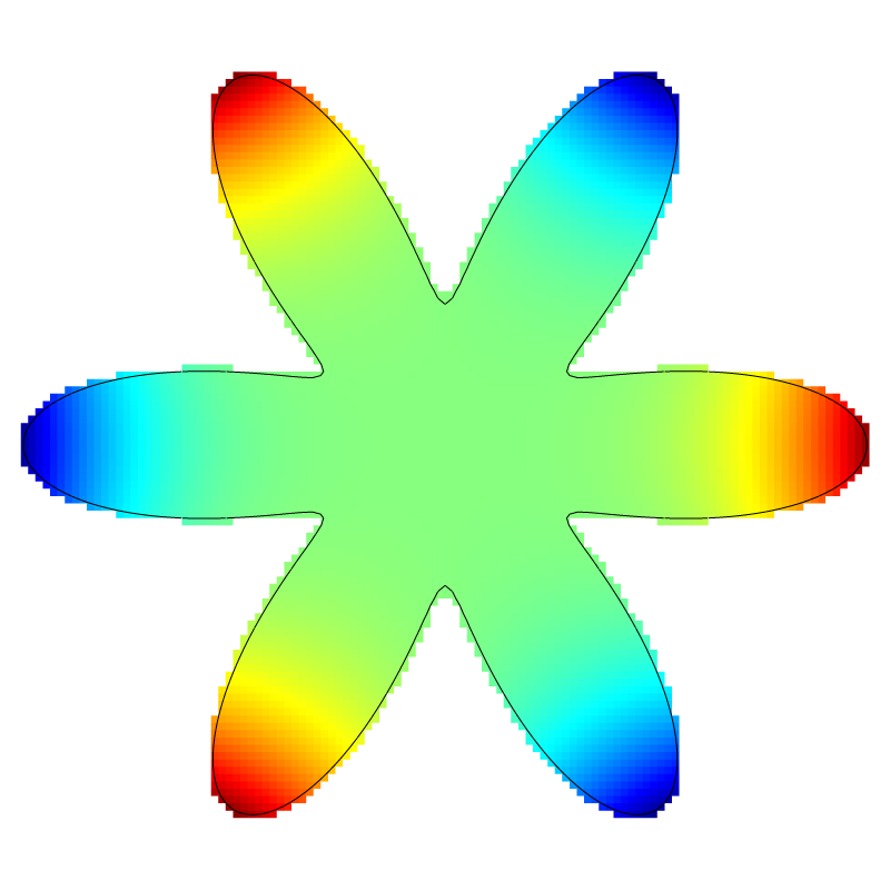
Solution for l=7

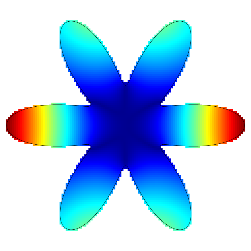
Error for l=7

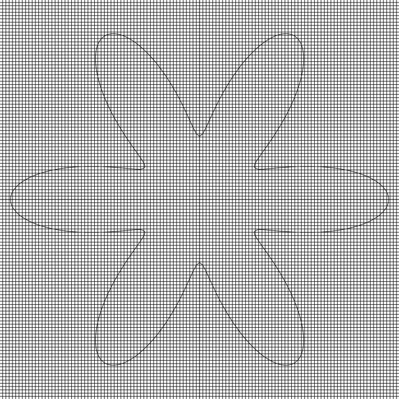
Mesh for l=7

Errors

set terminal svg font ",16"
set key bottom left spacing 1.1
set xtics 32,4,4096
set grid ytics
set ytics format "%.0e" 1.e-12,100,1.e2 
set xlabel 'N'
set ylabel '||res||_{inf}'
set xrange [32:4096]
set yrange [1.e-7:1.e1]
set logscale
plot 'out' u 1:3 w p ps 1.25 pt 7 lc rgb "black" t 'cut-cells', \
     ''    u 1:2 w p ps 1.25 pt 5 lc rgb "blue" t 'full cells'

Maximum truncation error (residual) (script)

set ylabel '||error||_{1}'
set yrange [1.e-10:1.e-3]
plot 'log' u 1:4 w p ps 1.25 pt 7 lc rgb "black" t 'cut-cells', \
     ''    u 1:6 w p ps 1.25 pt 5 lc rgb "blue" t 'full cells', \
     ''    u 1:2 w p ps 1.25 pt 2 lc rgb "red" t 'all cells'

Average error convergence (script)

set ylabel '||error||_{inf}'
plot '' u 1:5 w p ps 1.25 pt 7 lc rgb "black" t 'cut-cells', \
     '' u 1:7 w p ps 1.25 pt 5 lc rgb "blue" t 'full cells', \
     '' u 1:3 w p ps 1.25 pt 2 lc rgb "red" t 'all cells'

Maximum error convergence (script)

Order of convergence

Johansen and Collela, 1998 determined the following estimates for the residual, or truncation error:

for full cells, even though gradients at the faces of the cell are estimated with an O\left(\Delta^2\right) accuracy, the standard cancellation of the error when using cell-centered values to discretize the Laplacian gives: \displaystyle \mathrm{res}_f \sim \Delta^2
for cut-cells, because the gradients on the faces of the cell and the embedded boundary are estimated with an O\left(\Delta^2\right) accuracy, but the error doesn’t cancel out in the Laplacian, we have: \displaystyle \mathrm{res}_p \sim \frac{\Delta}{c_s}

We recover here the expected order of convergence. Note that if we do not account for the neighboring face fractions when computing the fluxes on the faces of each cut-cell, this leads to an O\left(1\right) error in the Laplacian.

reset
set terminal svg font ",16"
set key bottom right spacing 1.1
set xtics 32,4,4096
set ytics -4,1,4
set grid ytics
set xlabel 'N'
set ylabel 'Order of ||res||_{inf}'
set xrange [32:4096]
set yrange [-4:4.5]
set logscale x

# Asymptotic order of convergence

ftitle(b) = sprintf(", asymptotic order n=%4.2f", -b);
Nmin = log(1024);

f1(x) = a1 + b1*x; # cut-cells
f2(x) = a2 + b2*x; # full cells
f3(x) = a3 + b3*x; # all cells

fit [Nmin:*][*:*] f1(x) '< sort -k 1,1n out' u (log($1)):(log($3)) via a1,b1; # cut-cells 
fit [Nmin:*][*:*] f2(x) '< sort -k 1,1n out' u (log($1)):(log($2)) via a2,b2; # full cells

plot '< sort -k 1,1n out | awk -f ../data/order-res.awk' u 1:3 w lp ps 1.25 pt 7 lc rgb "black" t 'cut-cells'.ftitle(b1), \
     '< sort -k 1,1n out | awk -f ../data/order-res.awk' u 1:2 w lp ps 1.25 pt 5 lc rgb "blue" t 'full cells'.ftitle(b2)

Order of convergence of the maximum residual (script)

Johansen and Collela, 1998 also determined the following estimates for the error of the solution of the Poisson problem:

for full cells: \displaystyle \mathrm{err}_f \sim \Delta^2
for cut-cells, when using Neumann boundary conditions: \displaystyle \mathrm{err}_p \sim \Delta^2
for cut-cells, when using Dirichlet boundary conditions: \displaystyle \mathrm{err}_p \sim \Delta^3

We recover here the expected orders of convergence. Note that when using mesh adaptation, the order of convergence of both the residual and the error are determined by the order of the prolongataion/refinement functions, which are second-order accurate in Basilisk. However, in the complex “convex” geometry presented here, the restriction operation requires the user to input an embed_gradient to maintain second-order accuracy.

set ylabel 'Order of ||error||_{1}'

# Asymptotic order of convergence

fit [Nmin:*][*:*] f1(x) '< sort -k 1,1n log' u (log($1)):(log($4)) via a1,b1; # cut-cells 
fit [Nmin:*][*:*] f2(x) '< sort -k 1,1n log' u (log($1)):(log($6)) via a2,b2; # full-cells
fit [Nmin:*][*:*] f3(x) '< sort -k 1,1n log' u (log($1)):(log($2)) via a3,b3; # all cells

plot '< sort -k 1,1n log | awk -f ../data/order.awk' u 1:4 w lp ps 1.25 pt 7 lc rgb "black" t 'cut-cells'.ftitle(b1), \
     '< sort -k 1,1n log | awk -f ../data/order.awk' u 1:6 w lp ps 1.25 pt 5 lc rgb "blue" t 'full cells'.ftitle(b2), \
     '< sort -k 1,1n log | awk -f ../data/order.awk' u 1:2 w lp ps 1.25 pt 2 lc rgb "red" t 'all cells'.ftitle(b3)

Order of convergence of the average error (script)

set ylabel 'Order of ||error||_{inf}'

# Asymptotic order of convergence

fit [Nmin:*][*:*] f1(x) '< sort -k 1,1n log' u (log($1)):(log($5)) via a1,b1; # cut-cells 
fit [Nmin:*][*:*] f2(x) '< sort -k 1,1n log' u (log($1)):(log($7)) via a2,b2; # full-cells
fit [Nmin:*][*:*] f3(x) '< sort -k 1,1n log' u (log($1)):(log($3)) via a3,b3; # all cells

plot '< sort -k 1,1n log | awk -f ../data/order.awk' u 1:5 w lp ps 1.25 pt 7 lc rgb "black" t 'cut-cells'.ftitle(b1), \
     '< sort -k 1,1n log | awk -f ../data/order.awk' u 1:7 w lp ps 1.25 pt 5 lc rgb "blue" t 'full cells'.ftitle(b2), \
     '< sort -k 1,1n log | awk -f ../data/order.awk' u 1:3 w lp ps 1.25 pt 2 lc rgb "red" t 'all cells'.ftitle(b3)

Order of convergence of the maximum error (script)

References

[johansen1998]

Hans Johansen and Phillip Colella. A cartesian grid embedded boundary method for poisson’s equation on irregular domains. Journal of Computational Physics, 147(1):60–85, 1998. [ .pdf ]