sandbox/ghigo/src/test-navier-stokes/sphere-oscillating.c
Flow past a oscillating sphere for Re=40 and St=3.2
This test case is based on the numerical work of Mei, 1994 and is the 3D counterpart of the test case cylinder-oscillating.c. We reproduce here the results of Mei, 1994, Wang et al., 2010 and Schneiders et al., 2013. The authors studied the flow induced by the sinusoidal oscillation of a sphere in the x-direction.
We solve here the Navier-Stokes equations and add the sphere using an embedded boundary.
#include "grid/octree.h"
#include "../myembed.h"
#include "../mycentered.h"
#include "../myembed-moving.h"
#include "../myperfs.h"
#include "view.h"
Reference solution
#define d    (1.)
#define Re   (40.) // Particle Reynolds number
#define p_w0 (3.2) // Particle pulsation
#define uref (1.) // Reference velocity, uref
#define tref (min ((d)/(uref), 2.*M_PI/(p_w0))) // Reference time, tref=min (d/u, 2pi/w)
We define the sphere’s imposed motion.
#define p_acceleration(t,w) ((w)*cos((w)*(t))) // Particle acceleration
#define p_velocity(t,w)     (sin((w)*(t))) // Particle velocity
#define p_displacement(t,w) (-1./(w)*cos((w)*(t))) // Particle displacement
We also define the shape of the domain.
#define sphere(x,y,z) (sq ((x)) + sq ((y)) + sq ((z)) - sq ((d)/2.))

void p_shape (scalar c, face vector f, coord p)
{
  vertex scalar phi[];
  foreach_vertex()
    phi[] = (sphere ((x - p.x),
		     (y - p.y),
		     (z - p.z)));
  boundary ({phi});
  fractions (phi, c, f);
  fractions_cleanup (c, f,
		     smin = 1.e-14, cmin = 1.e-14);
}
Setup
We need a field for viscosity so that the embedded boundary metric can be taken into account.
face vector muv[];We define the mesh adaptation parameters and vary the maximum level of refinement.
#define lmin (5) // Min mesh refinement level (l=5 is 2pt/d)
#define cmax (1.e-2*(uref)) // Absolute refinement criteria for the velocity field
int lmax = 8; // Max mesh refinement level (l=8 is 16pt/d)

int main ()
{
The domain is 16\times 16\times 16.
We set the maximum timestep.
DT = 1.e-2*(tref);We set the tolerance of the Poisson solver.
  TOLERANCE    = 1.e-6;
  TOLERANCE_MU = 1.e-6*(uref);

  for (lmax = 8; lmax <= 10; lmax++) {
We initialize the grid.
Boundary conditions
We give boundary conditions for the face velocity to “potentially” improve the convergence of the multigrid Poisson solver.
uf.n[left]   = 0;
uf.n[right]  = 0;
uf.n[bottom] = 0;
uf.n[top]    = 0;
Properties
event properties (i++)
{
  foreach_face()
    muv.x[] = (uref)*(d)/(Re)*fm.x[];
  boundary ((scalar *) {muv});
}
Initial conditions
We set the viscosity field in the event properties.
mu = muv;We use “third-order” face flux interpolation.
#if ORDER2
for (scalar s in {u, p, pf})
s.third = false;
#else
for (scalar s in {u, p, pf})
s.third = true;
#endif // ORDER2We use a slope-limiter to reduce the errors made in small-cells.
#if SLOPELIMITER
for (scalar s in {u}) {
s.gradient = minmod2;
}
#endif // SLOPELIMITER
#if TREEWhen using TREE and in the presence of embedded boundaries, we should also define the gradient of u at the cell center of cut-cells.
#endif // TREEWe initialize the embedded boundary.
We first define the sphere’s initial position.
p_p.x = (p_displacement(0., (p_w0)));
#if TREEWhen using TREE, we refine the mesh around the embedded boundary.
astats ss;
int ic = 0;
do {
ic++;
p_shape (cs, fs, p_p);
ss = adapt_wavelet ({cs}, (double[]) {1.e-30},
maxlevel = (lmax), minlevel = (1));
} while ((ss.nf || ss.nc) && ic < 100);
#endif // TREE
p_shape (cs, fs, p_p);We initialize the particle’s speed and acceleration.
p_au.x = (p_acceleration (0., (p_w0)));
p_u.x = (p_velocity (0., (p_w0)));
}Embedded boundaries
The particle’s position is advanced to time t + \Delta t.
event advection_term (i++)
{
p_au.x = (p_acceleration (t + dt, (p_w0)));
p_u.x = (p_velocity (t + dt, (p_w0)));
p_p.x = (p_displacement (t + dt, (p_w0)));
}We verify here that the velocity and pressure gradient boundary conditions are correctly computed.
event check (i++)
{
foreach() {
if (cs[] > 0. && cs[] < 1.) {
// Normal pointing from fluid to solid
coord b, n;
embed_geometry (point, &b, &n);
// Velocity
bool dirichlet;
double ub;
ub = u.x.boundary[embed] (point, point, u.x, &dirichlet);
assert (dirichlet);
assert (ub -
p_u.x == 0.); ub = u.y.boundary[embed] (point, point, u.y, &dirichlet);
assert (dirichlet);
assert (ub -
p_u.y == 0.); ub = u.z.boundary[embed] (point, point, u.y, &dirichlet);
assert (dirichlet);
assert (ub -
p_u.z == 0.);
// Pressure gradient
bool neumann;
double pb; pb = p.boundary[embed] (point, point, p, &neumann);
assert (!neumann);
assert (pb +
rho[]/(cs[] + SEPS)*(p_au.x*n.x + p_au.y*n.y+ p_au.z*n.z) == 0.);
// Pressure gradient
double gb; gb = g.x.boundary[embed] (point, point, g.x, &dirichlet);
assert (dirichlet);
assert (gb - p_au.x == 0.); gb = g.y.boundary[embed] (point, point, g.y, &dirichlet);
assert (dirichlet);
assert (gb - p_au.y == 0.); gb = g.z.boundary[embed] (point, point, g.z, &dirichlet);
assert (dirichlet);
assert (gb - p_au.z == 0.);
}
}
}Adaptive mesh refinement
#if TREE
event adapt (i++)
{
adapt_wavelet ({cs,u}, (double[]) {1.e-2,(cmax),(cmax),(cmax)},
maxlevel = (lmax), minlevel = (1));We do not need here to reset the embedded fractions to avoid interpolation errors on the geometry as the is already done when moving the embedded boundaries. It might be necessary to do this however if surface forces are computed around the embedded boundaries.
}
#endif // TREEOutputs
double CD = 0., CLy = 0., CLz = 0.;
event init (i = 0)
{
CD = 0., CLy = 0., CLz = 0.;
}
event coeffs (i++; t <= 2.*2.*M_PI/(p_w0))
{
coord Fp, Fmu;
embed_force (p, u, mu, &Fp, &Fmu);
CD = (Fp.x + Fmu.x)/(0.5*sq ((uref))*pi*sq ((d)/2.));
CLy = (Fp.y + Fmu.y)/(0.5*sq ((uref))*pi*sq ((d)/2.));
CLz = (Fp.z + Fmu.z)/(0.5*sq ((uref))*pi*sq ((d)/2.));
char name1[80];
sprintf (name1, "level-%d.dat", lmax);
static FILE * fp = fopen (name1, "w");
fprintf (fp, "%d %g %g %d %d %d %d %d %d %g %g %g %g %g %g %g %g %g\n",
i, t/(2.*M_PI/(p_w0)), dt/(2.*M_PI/(p_w0)),
mgp.i, mgp.nrelax, mgp.minlevel,
mgu.i, mgu.nrelax, mgu.minlevel,
mgp.resb, mgp.resa,
mgu.resb, mgu.resa,
p_p.x/(d), p_u.x/(uref),
CD, CLy, CLz);
fflush (fp);
}
event logfile (t = end)
{
norm nx = normf(u.x), ny = normf(u.y), np = normf(p);
fprintf (stderr, "%d %d %g %g %g %d %d %d %d %d %d %g %g %g %g %g %g %g %g %g %g %g %g %g\n",
(lmax), (1 << (lmax)), (d)/((L0)/(1 << (lmax))),
t/(2.*M_PI/(p_w0)), dt/(2.*M_PI/(p_w0)),
mgp.i, mgp.nrelax, mgp.minlevel,
mgu.i, mgu.nrelax, mgu.minlevel,
mgp.resb, mgp.resa,
mgu.resb, mgu.resa,
CD, CLy, CLz,
nx.avg, nx.max, ny.avg, ny.max, np.avg, np.max
);
fflush (stderr);
}Snapshots
#if SNAP
event snapshot (t = {2.*M_PI/(p_w0)*(1.), 2.*M_PI/(p_w0)*(1. + 96./360.),
		     2.*M_PI/(p_w0)*(1. + 192./360.), 2.*M_PI/(p_w0)*(1. + 288./360.)})
{
  int phase = max(0, floorf ((t/(2.*M_PI/(p_w0)) - 1.)*360));

  scalar omega[];
  vorticity (u, omega);
  boundary ({omega});

  char name2[80];
We first plot the entire domain.
  view (fov = 20, camera = "front",
	tx = 0., ty = 0.,
	bg = {1,1,1},
	width = 800, height = 800);

  draw_vof ("cs", "fs", lw = 5);
  cells ();
  sprintf (name2, "mesh-level-%d-phi-%d.png", lmax, phase);
  save (name2);

  draw_vof ("cs", "fs", filled = -1, lw = 5);
  squares ("u.x", map = cool_warm);
  sprintf (name2, "ux-level-%d-phi-%d.png", lmax, phase);
  save (name2);

  draw_vof ("cs", "fs", filled = -1, lw = 5);
  squares ("u.y", map = cool_warm);
  sprintf (name2, "uy-level-%d-phi-%d.png", lmax, phase);
  save (name2);

  draw_vof ("cs", "fs", filled = -1, lw = 5);
  squares ("p", map = cool_warm);
  sprintf (name2, "p-level-%d-phi-%d.png", lmax, phase);
  save (name2);

  draw_vof ("cs", "fs", filled = -1, lw = 5);
  squares ("omega", map = cool_warm);
  sprintf (name2, "omega-level-%d-phi-%d.png", lmax, phase);
  save (name2);
We then zoom on the sphere.
  view (fov = 6, camera = "front",
	tx = 0., ty = 0., bg = {1,1,1},
	width = 800, height = 600);

  draw_vof ("cs", "fs", lw = 5);
  cells ();
  sprintf (name2, "mesh-zoom-level-%d-phi-%d.png", lmax, phase);
  save (name2);

  draw_vof ("cs", "fs", lw = 5);
  squares ("u.x", map = cool_warm);
  sprintf (name2, "ux-zoom-level-%d-phi-%d.png", lmax, phase);
  save (name2);

  draw_vof ("cs", "fs", lw = 5);
  squares ("u.y", map = cool_warm);
  sprintf (name2, "uy-zoom-level-%d-phi-%d.png", lmax, phase);
  save (name2);

  draw_vof ("cs", "fs", filled = -1, lw = 5);
  squares ("p", map = cool_warm);
  sprintf (name2, "p-zoom-level-%d-phi-%d.png", lmax, phase);
  save (name2);

  draw_vof ("cs", "fs", filled = -1, lw = 5);
  squares ("omega", map = cool_warm);
  sprintf (name2, "omega-zoom-level-%d-phi-%d.png", lmax, phase);
  save (name2);
}
#endif // SNAP
Results
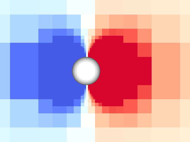
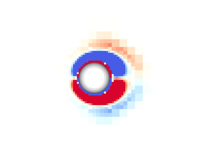
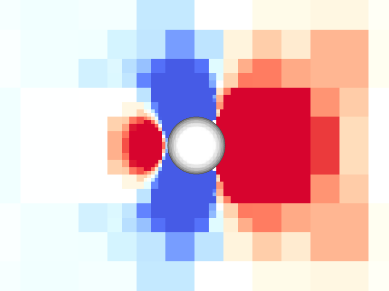
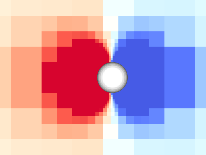
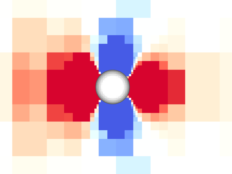
Pressure and vorticity in the xy-plane for level = 8


Periodicity
We first plot the time evolution of the drag and lift coefficients and verify that the flow has reached a periodic state after 1 cycle.
set terminal svg font ",16"
set key top right spacing 1.1
set xtics 0,0.5,10
set xlabel 't/T'
set ylabel 'C_D'
set xrange [0:2]
set yrange [-8:15]
plot 'level-8.dat'  u 2:16 w l lw 2 lc rgb "blue"      t "Basilisk, l=8", \
     'level-9.dat'  u 2:16 w l lw 2 lc rgb "red"       t "Basilisk, l=9", \
     'level-10.dat' u 2:16 w l lw 2 lc rgb "sea-green" t "Basilisk, l=10"
set ylabel 'C_{Ly}'
set yrange[-0.05:0.05]
plot 'level-8.dat'  u 2:17 w l lw 2 lc rgb "blue"      t "Basilisk, l=8", \
     'level-9.dat'  u 2:17 w l lw 2 lc rgb "red"       t "Basilisk, l=9", \
     'level-10.dat' u 2:17 w l lw 2 lc rgb "sea-green" t "Basilisk, l=10"
{Ly}
{Ly}
set ylabel 'C_{Lz}'
set yrange[-0.05:0.05]
plot 'level-8.dat'  u 2:18 w l lw 2 lc rgb "blue"      t "Basilisk, l=8", \
     'level-9.dat'  u 2:18 w l lw 2 lc rgb "red"       t "Basilisk, l=9", \
     'level-10.dat' u 2:18 w l lw 2 lc rgb "sea-green" t "Basilisk, l=10"
{Lz}
{Lz}
set ylabel "dt/T"
set yrange [1.e-4:1e0]
set logscale y
plot 'level-8.dat'  u 2:3 w l lw 2 lc rgb 'blue'      t 'Basilisk, l=8', \
     'level-9.dat'  u 2:3 w l lw 2 lc rgb 'red'       t 'Basilisk, l=9', \
     'level-10.dat' u 2:3 w l lw 2 lc rgb 'sea-green' t 'Basilisk, l=10'
Comparison with the results of fig. 20 from Schneiders et al., 2013.
We next plot the drag coefficent C_D as a function of time \omega t / 2/\pi over the last period. We compare the results with those of fig. 20 from Schneiders et al., 2013.
set ylabel "C_D"
set xrange [0:1]
set yrange [-8:15]
unset logscale
plot '../data/Schneiders2013/Schneiders2013-fig20-CD.csv' u 1:2 w p pt 6 ps 0.7 lc rgb "black" \
     t "fig. 20, Schneiders et al., 2013", \
     'level-8.dat'  u ($2 - 1):16 w l lw 2 lc rgb "blue"      t "Basilisk, l=8", \
     'level-9.dat'  u ($2 - 1):16 w l lw 2 lc rgb "red"       t "Basilisk, l=9", \
     'level-10.dat' u ($2 - 1):16 w l lw 2 lc rgb "sea-green" t "Basilisk, l=10"