naca0015-pitching.c

Flow past a rapidly pitching NACA0015 airfoil at Re=10000

Flow past a rapidly pitching NACA0015 airfoil at Re=10000

This test case is inspired from the numerical work of Visbal et Shang., 1989. We reproduce here the results of Schneiders et al., 2013. The authors studied the laminar flow around a rapidly pitching NACA0015 airfoil using a adaptive grid where the smallest mesh size is equivalent to 2000pt/c (c is the NACA0015 airfoil chord length).

We solve here the Navier-Stokes equations and add the NACA0015 using an embedded boundary.

#include "grid/quadtree.h"
#include "../myembed.h"
#include "../mycentered.h"
#include "../myembed-moving.h"
#include "../myperfs.h"
#include "view.h"

Reference solution

#define chord (1.) // NACA0015 chord length
#define Re    (10000.) // Reynolds number based on the cord length
#define p_w0  (0.6) // Pitch rate
#define p_t0  (1.) // Pitch characteristic time
#define p_ts  (0.2) // Pitch start time
#define uref  (1.) // Reference velocity, uref
#define tref  (min ((p_t0), (chord)/(uref))) // Reference time, tref

We define the NACA0015 airfoil’s pitch pitching rate and shape.

#define p_angle(t,ts,tau,w) ((t) < (ts) ? 0 :				\
			     (w)*(((t) - (ts)) + (tau)/4.6*(exp(-4.6*((t) - (ts))/(tau)) - 1.))) // NACA0015 pitch angle
#define p_rotation(t,ts,tau,w) ((t) < (ts) ? 0 :			\
				(w)*(1. - exp(-4.6*((t) - (ts))/(tau)))) // NACA0015 pitch rotation rate
#define p_acceleration(t,ts,tau,w) ((t) < (ts) ? 0 :			\
				    (w)*4.6/(tau)*exp(-4.6*((t) - (ts))/(tau))) // NACA0015 pitch rotation rate

We also define the shape of the domain.

#define naca00xx(x,y,a) (sq (y) - sq (5.*(a)*(0.2969*sqrt   ((x))	\
					      - 0.1260*((x))		\
					      - 0.3516*sq   ((x))	\
					      + 0.2843*cube ((x))	\
					      - 0.1036*pow  ((x), 4.)))) // -0.1015 or -0.1036

void p_shape (scalar c, face vector f, coord p)
{
  // NACA0015 parameters
  double tt = 0.15;

  // Rotation parameters around the position p,
  // located at the position cc in the airfoil referential
  double theta = (p_angle (t + dt, (p_ts), (p_t0), (p_w0)));
  coord cc = {0.25*(chord), 0.};
  
  vertex scalar phi[];
  foreach_vertex() {
    
    // Coordinates with respect to the center of rotation of the airfoil p
    // where the head of the airfoil is identified as xrot = 0, yrot = 0
    double xrot = cc.x + (x - p.x)*cos (theta) - (y - p.y)*sin (theta);
    double yrot = cc.y + (x - p.x)*sin (theta) + (y - p.y)*cos (theta);
    
    if (xrot >= 0. && xrot <= (chord)) {
      
      // Camber line coordinates, adimensional
      double xc = xrot/(chord), yc = yrot/(chord), thetac = 0.;
      
      // Thickness
      phi[] = (naca00xx (xc, yc, tt*cos (thetac)));
    }
    else
      phi[] = 1.;
  }
  boundary ({phi});
  fractions (phi, c, f);
  fractions_cleanup (c, f,
		     smin = 1.e-14, cmin = 1.e-14);
}

Setup

We need a field for viscosity so that the embedded boundary metric can be taken into account.

face vector muv[];

We define the mesh adaptation parameters.

#define lmin (8) // Min mesh refinement level (l=8 is 4pt/c)
#define lmax (15) // Max mesh refinement level (l=15 is 512pt/c)
#define cmax (1.e-3*(uref)) // Absolute refinement criteria for the velocity field

int main ()
{

The domain is 64\times 64.

  L0 = 64.;
  size (L0);
  origin (-L0/2., -L0/2.);

We set the maximum timestep.

  DT = 1.e-2*(tref);

We set the tolerance of the Poisson solver.

  TOLERANCE    = 1.e-4;
  TOLERANCE_MU = 1.e-4*(uref);

We initialize the grid.

  N = 1 << (lmin);
  init_grid (N);

  run ();
}

Boundary conditions

We use inlet boundary conditions.

u.n[left] = dirichlet ((uref));
u.t[left] = dirichlet (0);
p[left]   = neumann (0);
pf[left]  = neumann (0);

u.n[right] = neumann (0);
u.t[right] = neumann (0);
p[right]   = dirichlet (0);
pf[right]  = dirichlet (0);

We give boundary conditions for the face velocity to “potentially” improve the convergence of the multigrid Poisson solver.

uf.n[left]   = (uref);
uf.n[bottom] = 0;
uf.n[top]    = 0;

Properties

event properties (i++)
{
  foreach_face()
    muv.x[] = (uref)*(chord)/(Re)*fm.x[];
  boundary ((scalar *) {muv});
}

Initial conditions

event init (i = 0)
{

We set the viscosity field in the event properties.

  mu = muv;

We use “third-order” face flux interpolation.

#if ORDER2
  for (scalar s in {u, p, pf})
    s.third = false;
#else
  for (scalar s in {u, p, pf})
    s.third = true;
#endif // ORDER2

We use a slope-limiter to reduce the errors made in small-cells.

#if SLOPELIMITER
  for (scalar s in {u, p, pf}) {
    s.gradient = minmod2;
  }
#endif // SLOPELIMITER
  
#if TREE

When using TREE and in the presence of embedded boundaries, we should also define the gradient of u at the cell center of cut-cells.

#endif // TREE

We initialize the embedded boundary.

As the angle of the NACA0015 profile depends on the timestep dt, we also initialize dt to avoid using an arbitrary large dt to initialize the embedded boundaries.

  dt = DT;

#if TREE

When using TREE, we refine the mesh around the embedded boundary.

  astats ss;
  int ic = 0;
  do {
    ic++;
    p_shape (cs, fs, p_p);
    ss = adapt_wavelet ({cs}, (double[]) {1.e-30},
			maxlevel = (lmax), minlevel = (1));
  } while ((ss.nf || ss.nc) && ic < 100);
#endif // TREE
  
  p_shape (cs, fs, p_p);

We initialize the particle’s speed and accelerating.

  p_w.x  = -(p_rotation     (0., (p_ts), (p_t0), (p_w0)));
  p_w.y  = p_w.x;
  p_aw.x = -(p_acceleration (0., (p_ts), (p_t0), (p_w0)));
  p_aw.y = p_aw.x;

We initialize the velocity.

  foreach() 
    u.x[] = cs[]*(uref);
  boundary ((scalar *) {u});
}

Embedded boundaries

The particle’s position is advanced to time t + \Delta t.

event advection_term (i++)
{
  p_aw.x = -(p_acceleration (t + dt, (p_ts), (p_t0), (p_w0)));
  p_aw.y = p_aw.x;
  p_w.x  = -(p_rotation     (t + dt, (p_ts), (p_t0), (p_w0)));
  p_w.y  = p_w.x;
}

#if TREE
event adapt (i++)
{
  adapt_wavelet ({cs,u}, (double[]) {1.e-2,(cmax),(cmax)},
  		 maxlevel = (lmax), minlevel = (1));

We do not need here to reset the embedded fractions to avoid interpolation errors on the geometry as the is already done when moving the embedded boundaries. It might be necessary to do this however if surface forces are computed around the embedded boundaries.

}
#endif // TREE

Outputs

event logfile (i++; t <= (p_ts) + 1.85*(p_t0))
{
  coord Fp, Fmu;
  embed_force (p, u, mu, &Fp, &Fmu);

  double CD = (Fp.x + Fmu.x)/(0.5*sq ((uref))*(chord));
  double CL = (Fp.y + Fmu.y)/(0.5*sq ((uref))*(chord));

  fprintf (stderr, "%d %g %g %d %d %d %d %d %d %g %g %g %g %g %g %g\n",
	   i, (t - (p_ts))/(p_t0), dt/(p_t0),
	   mgp.i, mgp.nrelax, mgp.minlevel,
	   mgu.i, mgu.nrelax, mgu.minlevel,
	   mgp.resb, mgp.resa,
	   mgu.resb, mgu.resa,
	   (p_angle(t, (p_ts), (p_t0), (p_w0)))/M_PI*180.,
	   CD, CL);
  fflush (stderr);
}

Surface pressure coefficient and vorticity

We compute here the distribution of the pressure coefficient C_p and vorticity \omega at the surface of the NACA0015 airfoil when it reaches the pitch angles \theta = 44,\, 55 approximately.

void cpout (FILE * fp)
{
  foreach(serial)
    if (cs[] > 0. && cs[] < 1.) {

      coord b, n;
      embed_geometry (point, &b, &n);
      double xe = x + b.x*Delta, ye = y + b.y*Delta;
      double theta = (p_angle(t, (p_ts), (p_t0), (p_w0)));
      coord cc = {0.25*(chord)};
      double xcord = cc.x + (xe - p_p.x)*cos (theta) - (ye - p_p.y)*sin (theta);

      fprintf (fp, "%g %g %g %g\n",
	       xcord, // 1
	       M_PI + atan2(ye - p_p.y, xe - p_p.x), // 2
	       embed_interpolate (point, p, b), // 3
	       embed_vorticity (point, u, b, n) // 4
	       ); 
      fflush (fp);
    }
}

event surface_profile (t = {(p_ts) + 1.4971*(p_t0),
			    (p_ts) + 1.8172*(p_t0)})
{
  int angle = ((p_angle (t, (p_ts), (p_t0), (p_w0)))/M_PI*180.);
  char name[80];
  sprintf (name, "cp-angle-%d-pid-%d", angle, pid());
  FILE * fp = fopen (name, "w");
  cpout (fp);
  fclose (fp);
}

Snapshots

We plot here the vorticity isolines when the NACA0015 airfoil reaches the pitch angles \theta = 44,\, 55 approximately to compare them with fig. 18 and 19 of Schneiders et al., 2013.

event snapshot (t = {0., (p_ts) + 1.4971*(p_t0),
		     (p_ts) + 1.8172*(p_t0)})
{
  int angle = ((p_angle (t, (p_ts), (p_t0), (p_w0)))/M_PI*180.);
  
  scalar omega[];
  vorticity (u, omega);
  
  char name2[80];

We first plot the entire domain.

  view (fov = 20, camera = "front",
	tx = 0., ty = 1.e-12,
	bg = {1,1,1},
	width = 800, height = 800);

  draw_vof ("cs", "fs", lw = 5);
  cells ();
  sprintf (name2, "mesh-angle-%d.png", angle);
  save (name2);
    
  draw_vof ("cs", "fs", filled = -1, lw = 5);
  squares ("u.x", map = cool_warm);
  sprintf (name2, "ux-angle-%d.png", angle);
  save (name2);

  draw_vof ("cs", "fs", filled = -1, lw = 5);
  squares ("u.y", map = cool_warm);
  sprintf (name2, "uy-angle-%d.png", angle);
  save (name2);

  draw_vof ("cs", "fs", filled = -1, lw = 5);
  squares ("p", map = cool_warm);
  sprintf (name2, "p-angle-%d.png", angle);
  save (name2);

  draw_vof ("cs", "fs", filled = -1, lw = 5);
  squares ("omega", map = cool_warm);
  sprintf (name2, "omega-angle-%d.png", angle);
  save (name2);

We then zoom on the particle.

  view (fov = 0.4, camera = "front",
	tx = -(p_p.x + 0.2)/L0, ty = -(p_p.y - 0.1)/L0,
	bg = {1,1,1},
	width = 800, height = 800);

  draw_vof ("cs", "fs", lw = 5);
  cells ();
  sprintf (name2, "mesh-zoom-angle-%d.png", angle);
  save (name2);

  draw_vof ("cs", "fs", lw = 5);
  squares ("u.x", map = cool_warm);
  sprintf (name2, "ux-zoom-angle-%d.png", angle);
  save (name2);

  draw_vof ("cs", "fs", lw = 5);
  squares ("u.y", map = cool_warm);
  sprintf (name2, "uy-zoom-angle-%d.png", angle);
  save (name2);

  draw_vof ("cs", "fs", filled = -1, lw = 5);
  squares ("p", map = cool_warm);
  sprintf (name2, "p-zoom-angle-%d.png", angle);
  save (name2);

  draw_vof ("cs", "fs", filled = -1, lw = 5);
  squares ("omega", map = cool_warm, min = -100, max = 100);
  sprintf (name2, "omega-zoom-angle-%d.png", angle);
  save (name2);
}

Results

Vorticity

We compare here the vorticity isolines with those of fig. 18 and 19 from Schneiders et al., 2013, obtained when the NACA0015 airfoil reaches the pitch angles \theta = 44,\, 55.

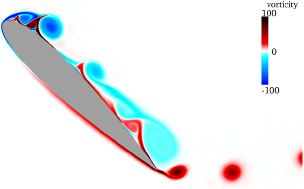
fig. 18 from Schneiders al., 2013

$Vorticity isolines for \theta = 44$

Vorticity isolines for \theta = 44

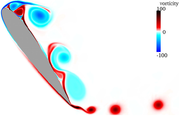
fig. 19 from Schneiders al., 2013

$Vorticity isolines for \theta = 55$

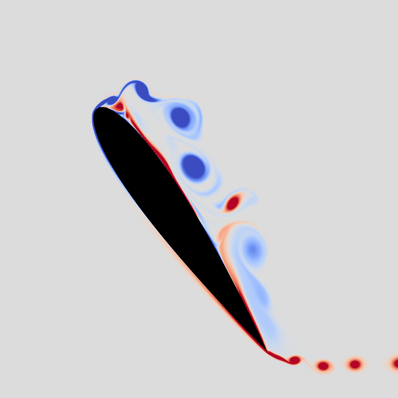
Vorticity isolines for \theta = 55

Drag and lift coefficients

We next plot the drag and lift coefficents C_D and C_L as a function of the pitch angle \theta. We compare the results with those of fig. 17 from Schneiders et al., 2013.

set terminal svg font ",16"
set key top right spacing 1.1
set xtics 0,10,100
set xlabel 'theta'
set ylabel 'C_{D,L}'
set xrange[0:55]
set yrange[0:6]
plot '../data/Schneiders2013/Schneiders2013-fig17-CD.csv' u 1:2 w p ps 0.7 pt 7 lc rgb "black" \
     t "fig. 17, Schneiders et al., 2013, C_D", \
     '../data/Schneiders2013/Schneiders2013-fig17-CL.csv' u 1:2 w p ps 0.7 pt 5 lc rgb "black" \
     t "fig. 17, Schneiders et al., 2013, C_L", \
     'log' u 14:15 w l lw 1.5 lc rgb "blue" t "Basilisk, C_D", \
     ''    u 14:16 w l lw 1.5 lc rgb "red"  t "Basilisk, C_L"

$Drag and lift coefficients C_D and C_L as a function of the angle \theta (script)$

Drag and lift coefficients C_D and C_L as a function of the angle \theta (script)

Surface pressure coefficient C_p around the NACA0015 airfoil

We finally plot the distribution of the pressure coefficient C_p at the surface of the NACA0015 airfoil when it reaches the pitch angles \theta = 44,\, 55 approximately.

set xtics 0,0.5,1
set xlabel 'x/c'
set ylabel 'C_p'
set xrange[0:1]
set yrange[-8:5]
plot '< cat cp-angle-44-pid-* | sort -k2,2' u 1:3 w p pt 7 ps 0.7 lc rgb "black" \
     t "theta = 44", \
     '< cat cp-angle-54-pid-* | sort -k2,2' u 1:3 w p pt 5 ps 0.7 lc rgb "blue" \
     t "theta = 55"

Pressure coefficient C_p at $= (script) {44,55}

References

[Schneiders2013]	L. Schneiders, D. Hartmann, M. Meinke, and W. Schroder. An accurate moving boundary formulation in cut-cell methods. Journal of Computational Physics, 235:786–809, 2013.
[Visbal1989]	M.R. Visbal and J.S. Shang. Investigation of the flow structure around a rapidly pitching airfoil. AIAA Journal, 27:1044–1051, 1989.