sandbox/ghigo/src/test-navier-stokes/hydrostatic2.c
Hydrostatic balance with refined embedded boundaries
This test case is related to the test case flow in a complex porous medium. We check that for a “closed pore” medium, hydrostatic balance can be recovered. This is not trivial in particular when the spatial resolution is variable, since pressure values need to be interpolated (at least) to second-order close to embedded boundaries. This behaviour depends on the restriction and prolongation operators used close to embedded boundaries.
#include "grid/quadtree.h"
#include "../myembed.h"
#include "../mycentered.h"
#include "view.h"
Geometry
We use a similar porous medium as in porous.c but with enough disks so that the pores are entirely closed.
void p_shape (scalar c, face vector f)
{
  int ns = 200;
  double xc[ns], yc[ns], R[ns];
  srand (0);
  for (int i = 0; i < ns; i++)
    xc[i] = 0.5*noise(), yc[i] = 0.5*noise(), R[i] = 0.02 + 0.04*fabs(noise());

  vertex scalar phi[];
  foreach_vertex() {
    phi[] = HUGE;
    for (double xp = -L0; xp <= L0; xp += L0)
      for (double yp = -L0; yp <= L0; yp += L0)
	for (int i = 0; i < ns; i++)
	  phi[] = intersection (phi[], (sq (x + xp - xc[i]) +
					sq (y + yp - yc[i]) -
					sq (R[i])));
  }
  boundary ({phi});
  fractions (phi, c, f);
  fractions_cleanup (c, f,
		     smin = 1.e-14, cmin = 1.e-14);
}
Setup
We define the mesh adaptation parameters.
#define lmin (6) // Min mesh refinement level
#define lmax (8) // Max mesh refinement level

int main()
{
The domain is 1\times 1.
  L0 = 1.;
  size (L0);
  origin (-L0/2., -L0/2.);
We set the maximum timestep.
DT = 1.e-2;We set the tolerance of the Poisson solver.
TOLERANCE = 1.e-6;We initialize the grid.
  N = 1 << (lmin);
  init_grid (N);

  run();
}
Boundary conditions
Properties
Initial conditions
We define the gravity acceleration vector.
  const face vector g[] = {1., 2.};
  a = g;
We use “third-order” face flux interpolation.
#if ORDER2
  for (scalar s in {u, p, pf})
    s.third = false;
#else
  for (scalar s in {u, p, pf})
    s.third = true;
#endif // ORDER2

#if TREE
When using TREE and in the presence of embedded boundaries, we should also define the gradient of u at the cell center of cut-cells.
#endif // TREEWe initialize the embedded boundary.
#if TREEWhen using TREE, we refine the mesh around the embedded boundary.
  astats ss;
  int ic = 0;
  do {
    ic++;
    p_shape (cs, fs);
    ss = adapt_wavelet ({cs}, (double[]) {1.e-2},
			maxlevel = (lmax), minlevel = (1));
  } while ((ss.nf || ss.nc) && ic < 100);
#endif // TREE

  p_shape (cs, fs);
We also define the volume fraction at the previous timestep csm1=cs.
csm1 = cs;We define the no-slip boundary conditions for the velocity.
  u.n[embed] = dirichlet (0);
  u.t[embed] = dirichlet (0);
  p[embed]   = neumann (0);

  uf.n[embed] = dirichlet (0);
  uf.t[embed] = dirichlet (0);
  pf[embed]   = neumann (0);
We finally give an initial guess for the pressure.
  foreach() {
    p[] = cs[] ? (g.x[]*x + g.y[]*y) : nodata; // exact pressure
    pf[] = p[];
  }
  boundary ((scalar *) {p, pf});
}
Embedded boundaries
Adaptive mesh refinement
Outputs
We only solve the Euler equations for a few time iterations.
We check the convergence rate and the norms of the velocity field (which should be negligible).
  assert (normf(u.x).max < 1.e-14 &&
	  normf(u.y).max < 1.e-14);

  fprintf (stderr, "%d %g %g %d %d %d %d %d %d %g %g %g %g %g %g\n",
	   i, t, dt,
	   mgpf.i, mgpf.nrelax, mgpf.minlevel,
	   mgp.i,  mgp.nrelax,  mgp.minlevel,
	   mgpf.resb, mgpf.resa,
	   mgp.resb,  mgp.resa,
	   normf(u.x).max, normf(u.y).max
	   );
}
Snapshots
event snapshot (t = end)
{
  view (fov = 20,
	tx = 0., ty = 0.,
	bg = {1,1,1},
	width = 800, height = 800);

  draw_vof ("cs", filled = -1, lw = 5, fc = {1,1,1});
  squares ("p", spread = -1);
  save ("p.png");
}
Results
The pressure is hydrostatic, in each of the pores.
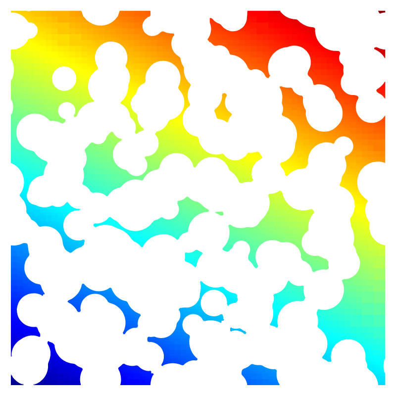
Pressure field