steady-state.c

Inviscid steady state
Code
Plots

Inviscid steady state

We solve the inviscid steady state of the 1D blood flow equations in an artery with variable properties. A steady state verifies the following system of equations:

\displaystyle \left\{ \begin{aligned} & Q = cst \\ & \frac{1}{2}\rho U^2 + p = cst\\ \end{aligned} \right.

From a numerical standpoint, these steady states are not easily obtained in an artery with variable properties. Indeed, a numerical error between the treatment of the flux and the topography source term can lead to the apparition of spurious velocities. This test case is therefore designed to test the ability of different well-balanced schemes to capture inviscid steady states.

Code

#include "grid/cartesian1D.h"
#include "bloodflow.h"

double R0 = 1.;
double K0 = 1.e4;
double L = 10.;

double DR = -1.e-1;
double XS = 3./10.*10.;
double XE = 7./10.*10.;

double DK = 1.e-1;
double XSS = 3./10.*10.;
double XEE = 7./10.*10.;

double SH = 1.e-1;
double AIN = 0., QIN = 0.;

scalar eq[];
double eq1, eq2, eqmax;

scalar am1[], qm1[];
scalar ecva[], ecvq[];

int ihr = 0;

double celerity (double a, double k) {

  return sqrt(0.5*k*sqrt(a));
}

int main() {

  origin (0., 0.);
  L0 = L;

  AIN = pi*pow(R0*(1 + SH), 2.);
  QIN = SH*AIN*celerity(AIN, K0);

  ihr = 0;
  for (ihr = 0; ihr <= 2; ihr ++) {
    for (N = 32; N <= 256; N *= 2) {

      eq1 = eq2 = eqmax = 0.;
    
      run();

      printf ("eq%d, %d, %g, %g, %g\n", ihr, N, eq1/QIN,
	      sqrt(eq2)/QIN, eqmax/QIN);
    }
  }
  
  return 0; 
}

q[left] = dirichlet(QIN);

event defaults (i=0) {

  gradient = order1;
  if (ihr == 0) riemann = hll_hr;
  else if (ihr == 1) riemann = hll_hrls;
  else if (ihr == 2) riemann = hll_glu;
}

event init (i=0) {
  
  foreach() {
    k[] = K0*(XSS <= x && x<=XEE ?
	      1. + DK/2.*(1 + cos(pi + 2.*pi*
				  (x - XSS)/(XEE - XSS))) :
	      1.);
    a0[] = pi*pow(R0, 2.)*pow(XS <= x && x <= XE ?
			      1. + DR/2.*(1 + cos(pi + 2.*pi*
						  (x - XS)/(XE - XS))) :
			      1., 2.);
    a[] = a0[];
    q[] = QIN;

    am1[] = a[];
    qm1[] = q[];
  }
}

event convergence (i++) {

  if (N == 128) {
    foreach() {
      ecva[] = (a[] - am1[])/a[];
      ecvq[] = (q[] - qm1[])/q[];
    }
  
    norm ncva = normf (ecva);
    norm ncvq = normf (ecvq);
    fprintf (stderr, "cv%d, %g, %.14f, %.14f\n", ihr, t, ncva.rms, ncvq.rms);

    foreach() { 
      am1[] = a[];
      qm1[] = q[];
    } 
  }
}
  
event field (t = end) {

  if (N == 128) {
    foreach() {
      fprintf (stderr, "%d, %g, %.6f, %.6f, %.6f, %.6f\n", ihr, x,
	       a0[]/(pi*R0*R0), k[]/K0, a[] - a0[], q[]) ;
    }
    fprintf (stderr, "\n\n") ;
  }
}

event error (t = end) {

  foreach() {
    eq[] = q[] - QIN;
  }
    
  norm nq = normf (eq);
  eq1 += nq.avg;
  eq2 += nq.rms*nq.rms;
  if (nq.max > eqmax)
    eqmax = nq.max;
}

event end (t = 1.5) {
  printf ("#Steady state test case completed\n") ;
}

Plots


reset

mycolors = "dark-blue red sea-green dark-violet orange brown4"
mypoints = '1 2 3 4 6 5'

set datafile separator ','
set style line 1 lt -1 lw 2 lc 'black'

set output 'A0K.png'
set xlabel 'x [cm]'
set ylabel 'Dimensionless arterial properties'
set key top right

plot '< grep ^0 log' u 2:3 w l ls 1 lc rgb word(mycolors, 1) t 'A_0/A_0(0)', \
     '< grep ^0 log' u 2:4 w l ls 1 lc rgb word(mycolors, 2) t 'K/K(0)'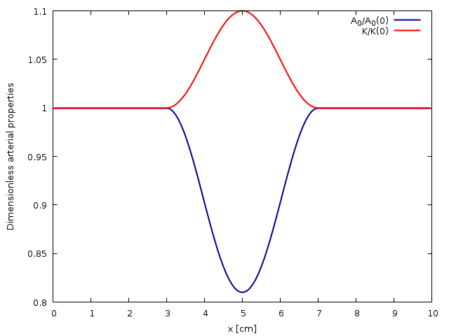

Spatial evolution of the cross-sectional area at rest A_0 and arterial wall rigidity K (script)


set output 'AmA0.png'
set xlabel 'x [cm]'
set ylabel 'A-A_0 [cm^2]'
set key center right

plot '< grep ^0 log' u 2:5 every 2 w p lt word(mypoints, 1) lc rgb word(mycolors, 1) ps 2 lw 1 t 'HR', \
     '< grep ^1 log' u 2:5 every 2 w p lt word(mypoints, 4) lc rgb word(mycolors, 2) ps 2 lw 1 t 'HR LS', \
     '< grep ^2 log' u 2:5 every 2 w p lt word(mypoints, 2) lc rgb word(mycolors, 3) ps 2 lw 1 t 'GLU'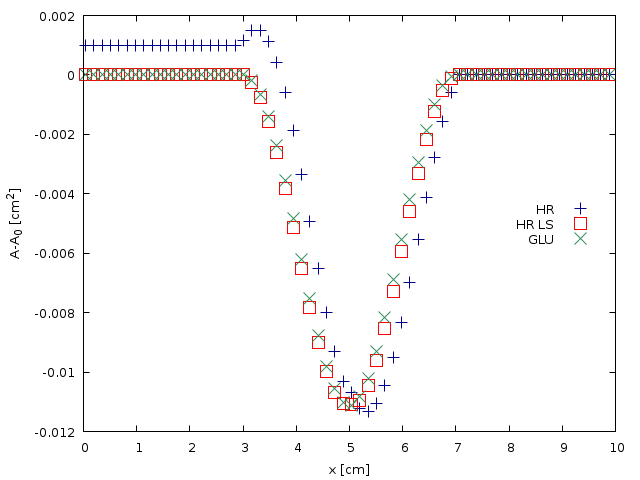

Spatial evolution of the cross-sectional area A-A_0 computed using the HR, HL-LS and GLU well-balanced schemes for N=128 (script)


a0 = pi
k0 = 1.e4
sh = 1.e-1
ain = a0*(1 + sh)**2.
qin = sh*ain*sqrt(0.5*k0*sqrt(ain))

set output 'Q.png'
set xlabel 'x [cm]'
set ylabel 'Q [cm^3/s]'
set key top right

plot qin w l ls 1 t 'Analytic', \
     '< grep ^0 log' u 2:6 every 2 w p lt word(mypoints, 1) lc rgb word(mycolors, 1) ps 2 lw 1 t 'HR', \
     '< grep ^1 log' u 2:6 every 2 w p lt word(mypoints, 4) lc rgb word(mycolors, 2) ps 2 lw 1 t 'HR LS', \
     '< grep ^2 log' u 2:6 every 2 w p lt word(mypoints, 2) lc rgb word(mycolors, 3) ps 2 lw 1 t 'GLU'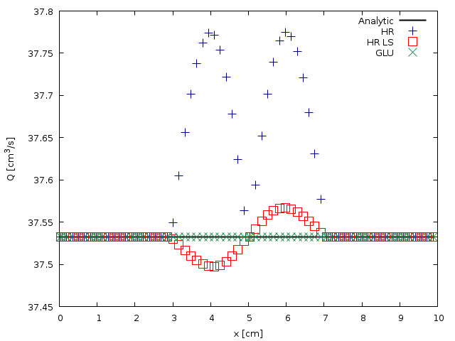

Spatial evolution of the flow rate Q computed using the HR, HL-LS and GLU well-balanced schemes for N=128 (script)

 
set output 'errCV.png'
set xlabel 't [s]'
set ylabel 'L_2 relative error norm'
set key top right
set logscale y

plot '< grep ^cv0 log' u 2:3 every ::1 w l ls 1 lc rgb word(mycolors, 1) t 'A', \
     '< grep ^cv0 log' u 2:4 every ::1 w l ls 1 lc rgb word(mycolors, 2) t 'Q'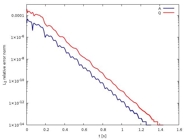

Time evolution of the relative L_2 error between two consecutive time steps for the cross-sectional area A and the flow rate Q computed using the HR well-balanced scheme (script)


set xtics 32,2,256
set logscale

ftitle(a,b) = sprintf('Order %4.2f', -b)
f1(x) = a1 + b1*x
f2(x) = a2 + b2*x
f3(x) = a3 + b3*x

fit f1(x) '< grep ^eq0 out' u (log($2)):(log($4)) via a1, b1
fit f2(x) '< grep ^eq1 out' u (log($2)):(log($4)) via a2, b2
fit f3(x) '< grep ^eq2 out' u (log($2)):(log($4)) via a3, b3

set output 'errQL2.png'
set xlabel 'N'
set ylabel '|Q|_2'
set key center right

set cbrange[1e-10:1e10]

plot '< grep ^eq0 out' u 2:4 w p lt word(mypoints, 1) lc rgb word(mycolors, 1) ps 3 lw 2 t 'HR, '.ftitle(a1, b1), \
     exp (f1(log(x))) ls 1 notitle, \
     '< grep ^eq1 out' u 2:4 w p lt word(mypoints, 2) lc rgb word(mycolors, 2) ps 3 lw 2 t 'HR LS, '.ftitle(a2, b2), \
     exp (f2(log(x))) ls 1 notitle, \
     '< grep ^eq2 out' u 2:4 w p lt word(mypoints, 3) lc rgb word(mycolors, 3) ps 3 lw 2 t 'GLU, '.ftitle(a3, b3), \
     exp (f3(log(x))) ls 1 notitle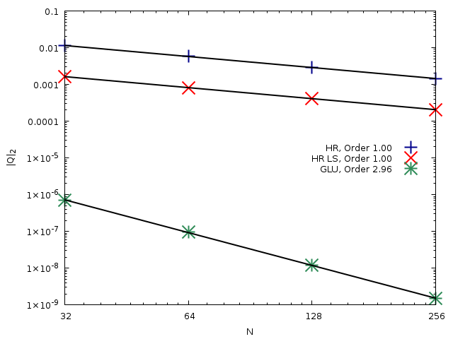

Comparison of the evolution of the L_2 relative error for the flow rate |Q|_2 with the number of cells N computed using the HR, HR-LS and GLU well-balanced schemes. (script)


fit f1(x) '< grep ^eq0 out' u (log($2)):(log($3)) via a1, b1
fit f2(x) '< grep ^eq0 out' u (log($2)):(log($4)) via a2, b2
fit f3(x) '< grep ^eq0 out' u (log($2)):(log($5)) via a3, b3

set output 'errQHR.png'
set xlabel 'N'
set ylabel 'Relative error norms'
set key top right

plot '< grep ^eq0 out' u 2:3 w p lt word(mypoints, 1) lc rgb word(mycolors, 1) ps 3 lw 2 t '|Q|_1, '.ftitle(a1, b1), \
     exp (f1(log(x))) ls 1 notitle, \
     '< grep ^eq0 out' u 2:4 w p lt word(mypoints, 2) lc rgb word(mycolors, 2) ps 3 lw 2 t '|Q|_2, '.ftitle(a2, b2), \
     exp (f2(log(x))) ls 1 notitle, \
     '< grep ^eq0 out' u 2:5 w p lt word(mypoints, 3) lc rgb word(mycolors, 3) ps 3 lw 2 t '|Q|_{max}, '.ftitle(a3, b3), \
     exp (f3(log(x))) ls 1 notitle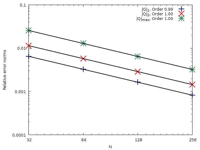

Evolution of the relative error norms for the flow rate with the number of cells N computed using the HR well-balanced scheme (script)