couette_torque.c

Couette flow between rotating cylinders + torque computation

Couette flow between rotating cylinders + torque computation

This case is a straight derivation of Stephane’s couette.

When computing forces (and torques!) on an embedded boundary, a common assumption is that velocity \mathbf{u} on the embedded interface is homogeneous, hence \mathbf{\nabla} \mathbf{u} \cdot \mathbf{t} = \mathbf{0} (see function embed_color_force and embed_color_torque from Arthur’s myembed.h).

This is not true if there is a tangential velocity component, such as, for the case of a rigid rotation (see derivation here).

Here we propose a simple test case, for the computation of torque on embedded boundaries having non-zero angular velocity: we test embedded boundaries by solving the (Stokes) Couette flow between two rotating cylinders.

We compare torques computed with our implementation with the one proposed in myembed.h

#include "grid/quadtree.h"
#include "ghigo/src/myembed.h"
#include "fpicella/src/compute_embed_color_force_torque_RBM.h"
#include "navier-stokes/centered.h"

#include "view.h"

‘color’ fields

These cs/fs fields are used to “mark” the outer and inner cylinder.

FILE * torque_output_file; // global file pointer

int main()
{

Space and time are dimensionless. This is necessary to be able to use the ‘mu = fm’ trick.

  size (1. [0]);
  DT = 1. [0];
  
  origin (-L0/2., -L0/2.);
  
  stokes = true;
  TOLERANCE = 1e-5;

	torque_output_file = fopen ("couette_torque.dat", "w");

  for (N = 16; N <= 256; N *= 2)
    run();
	
	fclose(torque_output_file);
}

scalar un[];

#define WIDTH 0.5

event init (t = 0) {

The viscosity is unity.

  mu = fm;

The geometry of the embedded boundary is defined as two cylinders of radii 0.5 and 0.25.

  solid (cs, fs, difference (sq(0.5) - sq(x) - sq(y),
			     sq(0.25) - sq(x) - sq(y)));

The outer cylinder is fixed and the inner cylinder is rotating with an angular velocity unity.

  u.n[embed] = dirichlet (x*x + y*y > 0.14 ? 0. : - y);
  u.t[embed] = dirichlet (x*x + y*y > 0.14 ? 0. :   x);
	// Inner cylinder has angular velocity +1, outer cylinder is held fixed.

We initialize the reference velocity field.

  foreach()
    un[] = u.y[];
}

Torque on a ROTATING embedded body.

We compute the torques on the OUTER and INNER cylinder using:

event compute_torque (i=-1) // set to -1 so to call the event at convergence
{

First, we compute the “colors”, marking the different cylinders.

	scalar csOUTER[];
	scalar csINNER[];
	face vector fsOUTER[];
	face vector fsINNER[];

  solid (csOUTER, fsOUTER, sq(0.5) - sq(x) - sq(y));
  solid (csINNER, fsINNER,         + sq(x) + sq(y) - sq(0.25));

	// allocate some auxiliary variables
  coord Tp, Tmu;
	coord center = {0.,0.,0.};
	coord OmegaINNER  = {1.,1.,1.}; // for the moment, it works ONLY in 2D!
	coord OmegaOUTER  = {0.,0.,0.}; // for the moment, it works ONLY in 2D!
	double rINNER = 0.25; // radius of the inner cylinder
	double rOUTER = 0.5; // radius of the outer cylinder
	// compute torques numerically
	// using ghigo/myembed.h functions
  embed_color_torque (p, u, mu, csOUTER, center, &Tp, &Tmu); // standard src/embed.h like approach
	double T_embed_OUTER = Tp.x + Tmu.x;
  embed_color_torque (p, u, mu, csINNER, center, &Tp, &Tmu); // standard src/embed.h like approach
	double T_embed_INNER = Tp.x + Tmu.x;
	// using fpicella's RBM function (accounting for rotating rigif boundary)
  embed_color_torque_RBM (p, u, mu, csOUTER, center, OmegaOUTER, rOUTER, &Tp, &Tmu);
	double T_embed_RBM_OUTER = Tp.x + Tmu.x;
  embed_color_torque_RBM (p, u, mu, csINNER, center, OmegaINNER, rINNER, &Tp, &Tmu);
	double T_embed_RBM_INNER = Tp.x + Tmu.x;
	// compute torques, analytically
	double nu = 1.; // viscosity;
  double T_ana_INNER = - 4*nu*M_PI*(OmegaINNER.x-OmegaOUTER.x)/(pow(rINNER,-2) - pow(rOUTER,-2));
	double T_ana_OUTER = -T_ana_INNER;
	fprintf(torque_output_file,
                "%04d %+6.5e %+6.5e %+6.5e %+6.5e %+6.5e %+6.5e\n",
                N,
                T_ana_INNER,       T_ana_OUTER,
                T_embed_INNER,     T_embed_OUTER,
                T_embed_RBM_INNER, T_embed_RBM_OUTER);
	fflush(torque_output_file);
}

We look for a stationary solution.

event logfile (t += 0.01; i <= 1000) {
  double du = change (u.y, un);
  if (i > 0 && du < 1e-6){
		event("compute_torque"); // so to compute torques only at convergence.
    return 1; /* stop */
	}
}

We compute error norms and display the angular velocity, pressure and error fields using bview.

#define powerlaw(r,N) (r*(pow(0.5/r, 2./N) - 1.)/(pow(0.5/0.25, 2./N) - 1.))

event profile (t = end)
{
  scalar utheta[], e[];
  foreach() {
    double theta = atan2(y, x), r = sqrt(x*x + y*y);
    if (cs[] > 0.) {
      utheta[] = - sin(theta)*u.x[] + cos(theta)*u.y[];
      e[] = utheta[] - powerlaw (r, 1.);
    }
    else
      e[] = p[] = utheta[] = nodata;
  }

  norm n = normf (e);
  fprintf (stderr, "%d %.3g %.3g %.3g %d %d %d %d %d\n",
	   N, n.avg, n.rms, n.max, i, mgp.i, mgp.nrelax, mgu.i, mgu.nrelax);
  dump();
  
  draw_vof ("cs", "fs", filled = -1, fc = {1,1,1});
  squares ("utheta", spread = -1);
  save ("utheta.png");

  draw_vof ("cs", "fs", filled = -1, fc = {1,1,1});
  squares ("p", spread = -1);
  save ("p.png");

  draw_vof ("cs", "fs", filled = -1, fc = {1,1,1});
  squares ("e", spread = -1);
  save ("e.png");

  if (N == 32)
    foreach() {
      double theta = atan2(y, x), r = sqrt(x*x + y*y);
      fprintf (stdout, "%g %g %g %g %g %g %g\n",
	       r, theta, u.x[], u.y[], p[], utheta[], e[]);
    }
}

Torques on both outer and inner cylinder.

At equilibrium, torques should be equal and opposite.

set xlabel 'N'
set ylabel 'T'

gnuplot: warning: Skipping data file with no valid points
gnuplot: x range is invalid

set grid
plot 'couette_torque.dat' u 1:2 w l t 'ana_INNER', 'couette_torque.dat' u 1:4 w l t 'embed_INNER', 'couette_torque.dat' u 1:6 w l t 'embed_RBM_INNER'

Torques (script)

Results

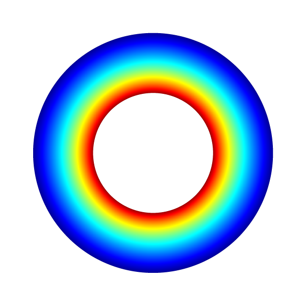
Angular velocity

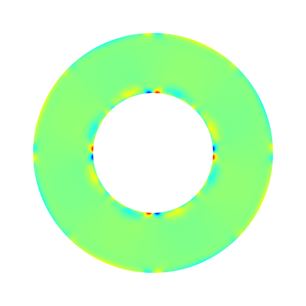
Pressure field

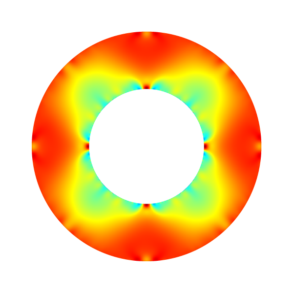
Error field

set xlabel 'r'
set ylabel 'u_theta'
powerlaw(r,N)=r*((0.5/r)**(2./N) - 1.)/((0.5/0.25)**(2./N) - 1.)
set grid
set arrow from 0.25, graph 0 to 0.25, graph 1 nohead
set arrow from 0.5, graph 0 to 0.5, graph 1 nohead
plot [0.2:0.55][-0.05:0.35]'out' u 1:6 t 'numerics', powerlaw(x,1.) t 'theory'

Velocity profile (N = 32) (script)

Convergence is close to second-order.

unset arrow
set xrange [*:*]
ftitle(a,b) = sprintf("%.3f/x^{%4.2f}", exp(a), -b)
f(x) = a + b*x
fit f(x) 'log' u (log($1)):(log($4)) via a,b
f2(x) = a2 + b2*x
fit f2(x) '' u (log($1)):(log($2)) via a2,b2
set xlabel 'Resolution'
set logscale
set xtics 8,2,1024
set ytics format "% .0e"
set grid ytics
set cbrange [1:2]
set xrange [8:512]
set ylabel 'Error'
set yrange [*:*]
set key top right
plot '' u 1:4 pt 6 t 'max', exp(f(log(x))) t ftitle(a,b), \
     '' u 1:2 t 'avg', exp(f2(log(x))) t ftitle(a2,b2)

Error convergence (script)