sandbox/acastillo/filaments/biot-savart.h

Vortex filament framework

For three-dimensional flows, a filamentary approach based on the cutoff theory exists in which the flow dynamics is described by the time evolution of lines.

\displaystyle \begin{aligned} \frac{d{\boldsymbol{\xi}}}{dt} = {\boldsymbol{U}}({\boldsymbol{\xi}},t) = {\boldsymbol{U}}_\infty + {\boldsymbol{U}}_{ind}({\boldsymbol{\xi}},t) \end{aligned} where {\boldsymbol{\xi}} is the position vector of the vortex filament, {\boldsymbol{U}} the velocity field, composed of an external field {\boldsymbol{U}}^\infty and a field {\boldsymbol{U}}({\boldsymbol{\xi}})^{ind} induced by the vortex filaments given by the Biot-Savart law: \displaystyle \begin{aligned} {\boldsymbol{U}}_{ind}({\boldsymbol{\xi}}) = \sum_j^{N} \frac{\Gamma_j}{4\pi} \int \frac{({\boldsymbol{\xi}}_j - {\boldsymbol{\xi}}) \times d{\boldsymbol{\tau}}_j}{\vert {\boldsymbol{\xi}}_j - {\boldsymbol{\xi}} \vert^2} \end{aligned} where the integrals cover each vortex filament defined by its circulation \Gamma_j, its position vector {\boldsymbol{\xi}}_j and its tangent vector {\boldsymbol{\tau}}_j.

On the vortex line, the Biot-Savart integral is singular, and the self-induced velocity diverges. To avoid this singularity, one has to assume a small but finite core size a. The self-induced motion is then obtained by an integral of the same form but without considering the interval [-\delta a,\delta a] around the singular point. The value of \delta depends on the vortex core model. Here, we shall assume a Gaussian vorticity profile for which \delta \approx 0.8736.

Vortex discretization

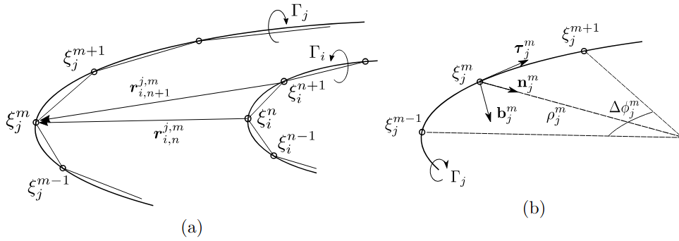
Discretization procedure of the vortex filaments. (a) Discretization in segments of two filaments of circulation \Gamma_i and \Gamma_j. (b) Arc of circle formed by three consecutive points of a discretized filament for the computation of the local contribution. Images taken from Durán Venegas & Le Dizès (2019)

We follow the vortex method approach described for instance in Leishman (2006). Each vortex filament is discretized in small segments in order to compute the velocity field and follow its displacement. In this way, the total induced velocity is computed from the contributions from the local auto-induced velocity and from the contributions from every vortex segment: as \displaystyle \begin{aligned} {\boldsymbol{U}}_{ind}({\boldsymbol{\xi}}_{i,m}) = {\boldsymbol{U}}_{loc}({\boldsymbol{\xi}}_{i,m}) + \sum_j^N \sum_n^{p_n} {\boldsymbol{U}}_{j,n}^{seg}({\boldsymbol{\xi}}_{i,m}) \end{aligned}

Local self-induced velocity

To determine the contribution to the velocity field at {\boldsymbol{\xi}}_i^m by the adjacent segments {\boldsymbol{\xi}}_i^{m-1} and {\boldsymbol{\xi}}_i^{m+1}, we replace the two segments by the arc of circle passing through ({\boldsymbol{\xi}}_i^{m-1},{\boldsymbol{\xi}}_i^m,{\boldsymbol{\xi}}_i^{m+1}) and use the cutoff formula \displaystyle \begin{aligned} {\boldsymbol{U}}^{loc}({\boldsymbol{\xi}}_{i,m}) = \frac{\Gamma_i}{4\pi\rho_i^m} \ln\left(\frac{\Delta\phi_i^m \rho_i^m}{\delta a} \right) {\boldsymbol{\hat{e}}}_b \end{aligned} where \rho_i^m and \hat{e}_b are the radius of curvature and the binormal unit vector at point {\boldsymbol{\xi}}_i^m, and \Delta\phi_i^m is the angle of the arc of circle.

In discretised form, these quantities are computed as follows. Let us introduce \displaystyle \begin{aligned} {\boldsymbol{u}} &= {\boldsymbol{\xi}}_{i,m-1} - {\boldsymbol{\xi}}_{i,m} \\ {\boldsymbol{v}} &= {\boldsymbol{\xi}}_{i,m+1} - {\boldsymbol{\xi}}_{i,m} \\ {\boldsymbol{w}} &= {\boldsymbol{u}}\times{\boldsymbol{v}} \end{aligned} and compute \displaystyle \begin{aligned} \frac{1}{\rho_i^m} &= \frac{2\vert {\boldsymbol{w}} \vert}{\vert {\boldsymbol{u}} \vert\vert {\boldsymbol{v}} \vert \vert {\boldsymbol{u}} - {\boldsymbol{v}}\vert}\\ \Delta\phi_i^m &= \frac{1}{2}\arccos{(1 - \frac{2\vert {\boldsymbol{w}} \vert^2}{\vert {\boldsymbol{v}} \vert^2 \vert {\boldsymbol{u}} - {\boldsymbol{v}}\vert^2} )} + \frac{1}{2}\arccos{(1 - \frac{2\vert {\boldsymbol{v}} \vert^2}{\vert {\boldsymbol{v}} \vert^2 \vert {\boldsymbol{u}} - {\boldsymbol{v}}\vert^2} )}\\ {\boldsymbol{\hat{e}}}_b &= \frac{{\boldsymbol{w}}}{\vert{\boldsymbol{w}}\vert} \end{aligned}

local_induced_velocity_segment: evaluates the velocity induced by 3-consecutive points

nseg

number of segments

A

corresponds to the points {\boldsymbol{\xi}}_i^{m-1}

B

corresponds to the points {\boldsymbol{\xi}}_i^{m}

C

corresponds to the points {\boldsymbol{\xi}}_i^{m+1}

a

corresponds to the core size a

velocity

corresponds to {\boldsymbol{U}}^{loc}({\boldsymbol{\xi}}_{m})

tangent

corresponds to {\boldsymbol{\hat{u}}}={\boldsymbol{u}}/\vert{\boldsymbol{u}}\vert

normal

corresponds to {\boldsymbol{\hat{v}}}={\boldsymbol{v}}/\vert{\boldsymbol{v}}\vert

binormal

corresponds to {\boldsymbol{\hat{w}}}={\boldsymbol{w}}/\vert{\boldsymbol{w}}\vert

curvature

corresponds to \kappa

dS

corresponds to the arclength \ell

Gamma

corresponds to the Circulation \Gamma

#include "PointTriangle.h"
void local_induced_velocity_segment(int n, coord *A, coord *B, coord *C, double *a, 
  coord *velocity, coord *tangent, coord *normal, coord *binormal, 
  double *curvature, double *dS, double Gamma=1.0) {
  for (int i = 0; i < n; i++) {
    // Compute the curvature of the arc of circle passing through points A, B
    // and C
    coord U = vecdiff(A[i],B[i]);
    coord V = vecdiff(C[i],B[i]);
    coord UV = vecdiff(U,V);
    coord W = vecdotproduct(U,V); 

    double norm_U = sqrt(vecdot(U,U));
    double norm_V = sqrt(vecdot(V,V));
    double norm_W = sqrt(vecdot(W,W));
    double norm_UV = sqrt(vecdot(UV,UV));    
    double denominator = norm_U * norm_V * norm_UV;
    curvature[i] = norm_W / denominator * 2;

    // Compute the angle of the arc
    double dT1 = acos(1 - sq(norm_U * curvature[i]) / 2);
    double dT2 = acos(1 - sq(norm_V * curvature[i]) / 2);
    double dT = (dT1 + dT2) / 2;

    // Compute the self-induced velocity
    const double delta = 0.8763;
    dS[i] = dT / curvature[i];
    double Uloc = -Gamma / (4 * pi) * curvature[i] * log(dS[i] / (a[i] * delta));

    // Compute the binormal unit vector    
    foreach_dimension(){
      tangent[i].x  =  U.x / norm_U;
      normal[i].x   =  V.x / norm_V;
      binormal[i].x =  W.x / norm_W;
      velocity[i].x = Uloc * binormal[i].x;
    }          
  }
}

leftCircularShift: shifts array one position to the left

void leftCircularShift(coord arr[], int size) {
  if (size <= 1) {
    return; // No shift needed for arrays of size 0 or 1
  }
  coord firstElement = arr[0];
  memmove(&arr[0], &arr[1], (size - 1) * sizeof(coord));
  arr[size - 1] = firstElement;
}

rightCircularShift: shifts array one position to the right

void rightCircularShift(coord arr[], int size) {
  if (size <= 1) {
    return; // No shift needed for arrays of size 0 or 1
  }
  coord lastElement = arr[size - 1];
  memmove(&arr[1], &arr[0], (size - 1) * sizeof(coord));
  arr[0] = lastElement;
}

local_induced_velocity: evaluates the local auto induced velocity of a filament

void local_induced_velocity(struct vortex_filament filament) {
  int nseg = filament.nseg;

  coord A[nseg], B[nseg], C[nseg];
  memcpy(A, filament.C, nseg * sizeof(coord));
  rightCircularShift(A, nseg);

  memcpy(B, filament.C, nseg * sizeof(coord));

  memcpy(C, filament.C, nseg * sizeof(coord));
  leftCircularShift(C, nseg);

  local_induced_velocity_segment(nseg, A, B, C, filament.a, filament.Ulocal, 
    filament.Tvec, filament.Nvec, filament.Bvec, filament.kappa, filament.s);
}

Contributions from non-local terms

Biot-Savart is discretised as \displaystyle \begin{aligned} {\boldsymbol{U}}_{j,n}^{seg}({\boldsymbol{\xi}}_{i,m}) = \frac{\Gamma_j}{4\pi} \frac{P}{Q} ({\boldsymbol{a}} \times {\boldsymbol{b}}) \end{aligned} where {\boldsymbol{a}} = {\boldsymbol{\xi}}_{j,n} - {\boldsymbol{\xi}}_{i,m}, {\boldsymbol{b}} = {\boldsymbol{\xi}}_{j,{n+1}} - {\boldsymbol{\xi}}_{i,m}, and \displaystyle \begin{aligned} P &= \frac{({\boldsymbol{a}}\cdot{\boldsymbol{b}}) - {\boldsymbol{a}}^2}{\vert{\boldsymbol{a}}\vert} + \frac{({\boldsymbol{a}}\cdot{\boldsymbol{b}}) - {\boldsymbol{b}}^2}{\vert{\boldsymbol{b}}\vert} \\ Q &= ({\boldsymbol{a}}\cdot{\boldsymbol{b}})^2 - {\boldsymbol{a}}^2 {\boldsymbol{b}}^2 \end{aligned}

In practice, we shall use \displaystyle \begin{aligned} {\boldsymbol{U}}_{j,n}^{seg}({\boldsymbol{\xi}}_{i,m}) &= \frac{\Gamma}{4\pi} \frac{ ({\boldsymbol{a}} \times {\boldsymbol{b}}) } { ({\boldsymbol{a}} \cdot {\boldsymbol{b}})^2 - \vert {\boldsymbol{b}} \vert^2 \vert {\boldsymbol{a}} \vert^2 \color{red} + \delta_a + \delta_b } \left[ \frac{ ({\boldsymbol{a}}\cdot{\boldsymbol{b}}) - \vert{\boldsymbol{a}}\vert^2 }{ \vert {\boldsymbol{a}} \vert + \color{red}\delta_a} + \frac{ ({\boldsymbol{a}}\cdot{\boldsymbol{b}}) - \vert{\boldsymbol{b}}\vert^2 } {\vert {\boldsymbol{b}} \vert + \color{red}\delta_b} \right] \end{aligned} Note that, the terms in red with \delta_a=\delta(x-{\boldsymbol{a}}^2) and \delta_b=\delta(x-{\boldsymbol{b}}^2) were included by Durán Venegas & Le Dizès (2019), to ensure that P/Q wont diverge and set {\boldsymbol{U}}_{j,n}^{seg}=0 when ({\boldsymbol{a}}\cdot{\boldsymbol{a}}) or ({\boldsymbol{b}}\cdot{\boldsymbol{b}}) are (close to) zero. Instead, the contributions from local auto-induction are obtained from the cut-off approach.

coord nonlocal_induced_velocity(coord target, struct vortex_filament source, double Gamma=1.0) {
  
  const double tol = 1e-8;
  int nseg = source.nseg;
  
  coord A[nseg], B[nseg];
  memcpy(A, source.C, nseg * sizeof(coord)); // a copy of C
  memcpy(B, source.C, nseg * sizeof(coord));
  leftCircularShift(B, nseg);
  
  coord velocity = {0.,0.,0.};
  for (int j = 0; j < nseg; j++){
    // Evaluate the position offsets
    coord a, b;
    foreach_dimension(){
      a.x = A[j].x - target.x;
      b.x = B[j].x - target.x;
    }
    coord c = vecdotproduct(a,b);

    // Dot product of vectors A and B
    double AB = vecdot(a,b);
    double A2 = vecdot(a,a);
    double B2 = vecdot(b,b);

    // Norms of vectors A and B (set to one if A=0 and/or B=0)      
    double corr_A = fabs(A2) < tol ? 1.0 : 0.0 ;
    double corr_B = fabs(B2) < tol ? 1.0 : 0.0 ;
    double A2q = sqrt(A2 + corr_A);
    double B2q = sqrt(B2 + corr_B);

    // Assemble the induced velocity components
    double P = (AB - A2)/A2q + (AB - B2)/B2q;
    double Q = sq(AB) - A2*B2 - (corr_A + corr_B)*(A2 + B2 - 2*AB);
            
    foreach_dimension(){
      velocity.x += (Gamma/(4*pi))*(P/Q)*c.x;
    }
  }
  return velocity;
}

void write_filament_state(FILE* fp, struct vortex_filament *filament) {
    // Check if the file pointer is valid
    if (fp == NULL) {
        fprintf(stderr, "Error: Invalid file pointer in write_filament_state.\n");
        return;
    }    
    int nseg = filament->nseg;
    for (int j = 0; j < nseg; j++) {
        fprintf(fp, "%g %d ", t, j);
        fprintf(fp, "%g %g %g ", filament->C[j].x,       filament->C[j].y,       filament->C[j].z);
        fprintf(fp, "%g %g %g ", filament->Ulocal[j].x,  filament->Ulocal[j].y,  filament->Ulocal[j].z);
        fprintf(fp, "%g %g %g ", filament->Uauto[j].x,   filament->Uauto[j].y,   filament->Uauto[j].z);
        fprintf(fp, "%g %g %g ", filament->Umutual[j].x, filament->Umutual[j].y, filament->Umutual[j].z);
        fprintf(fp, "%g %g %g ", filament->U[j].x,       filament->U[j].y,       filament->U[j].z);
        fprintf(fp, "%g \n", filament->a[j]);
    }
    fputs("\n", fp); 
}

References