sandbox/acastillo/faraday_waves_mixing/faraday.c
- Faraday waves in rectangular containers
- 1. General equations
- 2. Implementation in Basilisk
- 3. Outputs
- References
Faraday waves in rectangular containers
Faraday observed that a fluid layer of density \rho and depth h is unstable to a periodic vertical motion with amplitude a and frequency \omega, leading to the generation of standing waves oscillating with half the forcing frequency. For ideal fluids, Benjamin & Ursell (1954) showed this motion to be well described by a Matthieu equation in terms of the acceleration ratio a\omega^2/g — g being the standard gravity — and the frequency ratio (\omega/\omega_n)^2 — \omega_n being the frequency of small oscillations. They revealed unstable regions, or U-tongues, where the frequency of the solution is either isochronous (harmonic) of half-frequency (sub-harmonic). For small amplitudes, surface waves remain time-periodic and symmetrical with respect to the vertical plane. As the amplitude increases, the formation of flat-crested waves, dimpled waves, and wave breaking.
The interaction between a miscible and an immiscible fluid layer offers an interesting setting, where the properties of the internal layer evolve due to molecular diffusion and turbulent entrainment. Linden (1973) argued that discrete turbulent motions may transfer their kinetic energy into potential energy by deforming the interface and promoting mixing between the two layers. Over time, the mixing layer becomes both deeper and thicker, driven by two competing mechanisms:
the density contrast across the interface decreases as the near-surface region becomes increasingly homogeneous, reducing the energy required for irreversible mixing — a process reminiscent of penetrative convection.
the energy injected into the interface diminishes with distance from the free surface, analogous to the behaviour of impinging jets, rising plumes, or oscillating grid turbulence in stratified fluids.
Eventually, as the available energy decreases faster than the energy needed for mixing, the interface is bound to decouple from the surface dynamics and stall.
In this example, we investigate the interaction between a free surface and a miscible interface with a small density contrast through direct numerical simulations (DNS) of a simplified configuration shown below.
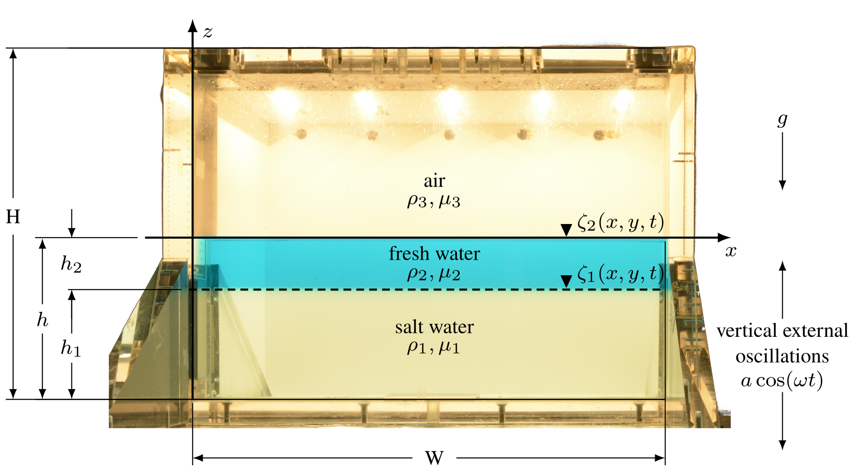
Figure 1: Experimental setup showing the cuboidal tank with inner dimensions W×H×D, the initial two-layer configuration, and forcing parameters.
Surface waves are generated by applying a periodic vertical oscillation—of amplitude a and frequency \omega—to the container. The response frequency is either \omega (harmonic) or \omega/2 (sub-harmonic). Depending on the external acceleration a\omega^2 we may observe a wavy, unbroken, free surface or a disconnected surface as in a breaking wave. Wave breaking can also lead to splashing droplets and jets from the collapse of large cavities, which inject fresh fluid into the stratified layer
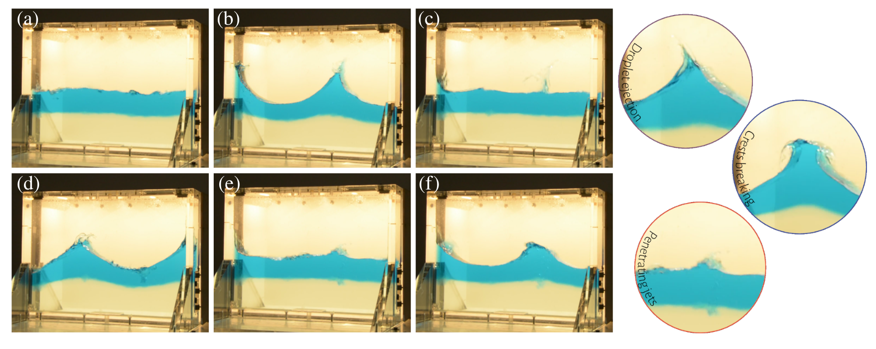
Figure 2: A large-amplitude standing wave interacting with a stratified layer, with light fluid shown in blue. Subfigures (a) to (f) depict snapshots taken at regular intervals over three periods *T = 2/. Insets in the right panel highlight characteristic features such as droplet ejection, crests breaking, and penetrating jets.
A representative example of the 3D simulations for a case with strong forcing and intermediate stratification is shown below:

1. General equations
1.1. Dimensional equations
We consider a system of two immiscible, incompressible fluids, each with density \rho_i, where the subscript i \in \lbrace 1; 2 \rbrace identifies the respective fluid. Here, \rho_2 denotes the density of the lighter fluid and \rho_1 > \rho_2 represents the denser fluid. The fluids are confined within a cuboidal container that is oscillated at frequency \omega and amplitude a along one of its principal axes, specifically the vertical direction. In a Cartesian coordinate frame \vec{x} = (x, y, z) moving with the container, the system is subjected to the ambient gravitational field g on top of the oscillatory acceleration, both of which act in the vertical z-direction.
This system is governed by the incompressible Navier-Stokes equations, which describe the dynamics of the velocity field \vec{U}_i(\vec{x},t) and the pressure P(\vec{x},t). For each phase, this yields:
\displaystyle \begin{aligned} \partial_t\vec{U}_{i} + \vec{U}_{i}\cdot(\nabla\vec{U}_{i}) &= -\frac{1}{\rho_i}\nabla\cdot\vec{\tau}_i - \vec{a}(t) \\ \partial_t\rho_{i} + \vec{U}_{i}\cdot(\nabla\rho_{i}) &= 0 \\ \nabla\cdot\vec{U}_{i} &= 0 \end{aligned}
which express the conservation of momentum, the conservation of mass and the incompressibility condition, respectively. The external acceleration is \vec{a}(t) = (g+a\omega^2\cos(\omega t))\vec{e}_z, and \vec{\tau}_i is the stress tensor:
\displaystyle \begin{aligned} \vec{\tau}_i = -P_i\vec{I} + \mu_i (\nabla\vec{U}_i+\nabla\vec{U}_i^T) + \gamma\kappa\delta_s(\vec{n}\otimes\vec{n}) \end{aligned}
where \mu_i, \gamma, \kappa, \delta_s, and \vec{n} represent the viscosity, surface tension coefficient, local curvature, a surface Dirac delta function, and the unit normal vector of the free surface, respectively. We may also write the viscous stress tensor \Pi_{\nu_i} = (\nabla \vec{U}_i + {\nabla \vec{U}_i}^T) and the effect of surface tension \vec{f}_\gamma = \kappa \delta_s \vec{n} for compactness.
Stratification is included using a (volumetric) concentration field C_i(\vec{x},t) \in [0, 1] governed by the transport equation:
\displaystyle \begin{aligned} \partial_t C_{i} + \vec{U}_{i}\cdot(\nabla C_{i}) &= -\nabla\cdot(\vec{J}_{i}) \end{aligned}
where \vec{J}_i is the concentration flux (see, for instance, Haroun et al. (2010); Marschall et al. (2012)).
The equations are coupled through the fluid properties. For the binary mixture, the viscosity is assumed constant (\mu_1 = \mu_\mathrm{salt~water} = \mu_\mathrm{fresh~water}). For small density contrasts, the density \rho_1 is taken as a linear function of C_1:
\displaystyle \begin{aligned} \rho_1(\vec{x},t) = C_1(\vec{x},t)\rho_\mathrm{1,max} + (1-C_1(\vec{x},t))\rho_\mathrm{1,min} \end{aligned}
1.2. Dimensionless equations
These variables, along with the spatial coordinate \vec{x} and time t, are nondimensionalized using the wavenumber k_n, acceleration g, and a reference density \rho_0 = (\rho_1 + \rho_2 )/2. Let us introduce the following dimensionless variables:
\displaystyle \begin{aligned} \vec{x}^* = x k_n, \quad t^* = t \sqrt{gk_n}, \quad \vec{U}_i^* = \frac{\vec{U}_i}{\sqrt{g / k_n}}, \quad P_i^* = \frac{P_i}{\rho_0 g / k_n}, \quad \rho_i^* = \frac{\rho_i}{\rho_0} \end{aligned}
The nondimensionalized governing equations become:
\displaystyle \begin{aligned} \partial_{t}\vec{U}_{1} + \vec{U}_{1}\cdot(\nabla\vec{U}_{1}) &= -\frac{1}{\rho_1}\nabla P_1 + \frac{1}{\mathrm{Re}} \nabla \cdot \Pi_{\nu_1} + \frac{2\mathcal{A}}{\mathrm{We}} \frac{\vec{f}_\gamma}{\rho_1} - \left(1 + \mathrm{Fr}\cos(t\omega/\omega_n)\right)\vec{e}_z, \\ \partial_{t}\vec{U}_{2} + \vec{U}_{2}\cdot(\nabla\vec{U}_{2}) &= - \frac{1}{\rho_2}\nabla P_2 + \frac{\Upsilon}{\mathrm{Re}} \nabla \cdot \Pi_{\nu_2} + \frac{2\mathcal{A}}{\mathrm{We}} \frac{\vec{f}_\gamma}{\rho_2} - \left(1 + \mathrm{Fr}\cos(t\omega/\omega_n)\right)\vec{e}_z, \\ \partial_{t}\rho_{i} + \vec{U}_{i}\cdot(\nabla\rho_{i}) &= 0 \\ \nabla\cdot\vec{U}_{i} &= 0, \\ \partial_{t}\vec{C}_{1} + \vec{U}_{1}\cdot(\nabla\vec{C}_{1}) &= \nabla \cdot \left(\frac{1}{\mathrm{Sc}\mathrm{Re}} \nabla\vec{C}_{1}\right) \\ \partial_{t}\vec{C}_{2} + \vec{U}_{2}\cdot(\nabla\vec{C}_{2}) &= \nabla \cdot \left(\frac{\Upsilon}{\mathrm{Sc}\mathrm{Re}} \nabla\vec{C}_{2}\right) \end{aligned}
where the ^* symbols are omitted for clarity and \omega_n = \sqrt{g k_0}. The key nondimensional parameters are:
- The Reynolds number: \mathrm{Re} = \sqrt{g/k_n^3}/\nu_1
- The Froude number: \mathrm{Fr} = a\omega^2/g
- The Weber number: \mathrm{We} = (\rho_1-\rho_2)g/k_n\gamma
- The Atwood number: \mathcal{A} = (\rho_1-\rho_2)/(\rho_1+\rho_2)
- The viscosity ratio: \Upsilon = \nu_2/\nu_1
- The Schmidt number: \mathcal{Sc} = \nu_1/\mathscr{D}
1.3. One-fluid formulation
In the one-fluid formulation, we may introduce a volume fraction field \phi_i(\vec{x},t), representing the spatial distributions of each fluid:
\displaystyle \begin{aligned} \phi_1(\vec{x},t) = \frac{V_1}{V_1+V_2}, \quad \phi_2(\vec{x},t) = \frac{V_2}{V_1+V_2}, \quad \phi_1(\vec{x},t) + \phi_2(\vec{x},t) = 1 \end{aligned}
In practice, we may use only the volume fraction of heavy fluid and drop the subscript. Since fluids are non-miscible, \phi(\vec{x},t) is either 0 or 1 everywhere but on the interface.
The renormalized density \rho is related to the volume fraction of heavy fluid \phi
\displaystyle \begin{aligned} \rho(\phi) = (1 + \mathcal{A})\phi + (1 - \mathcal{A})(1-\phi). \end{aligned}
Additionally, we introduce average velocity and pressure fields, \vec{U}=\phi\vec{U}_2 + (1-\phi)\vec{U}_1 and P=\phi P_2 + (1-\phi)P_1. Also, we introduce a viscous stress tensor \Pi_{\nu}=\phi\Pi_{\nu_2}+(1-\phi)\Upsilon\Pi_{\nu_1}. This yields
\displaystyle \begin{aligned} \partial_{t}\vec{U} + \vec{U}\cdot(\nabla\vec{U}) &= -\frac{1}{\rho(\phi)}\nabla P + \frac{1}{\mathrm{Re}} \nabla \cdot \Pi_{\nu} + \frac{2\mathcal{A}}{\mathrm{We}} \frac{\vec{f}_\gamma}{\rho(\phi)} - \left(1 + \mathrm{Fr}\cos(t)\right)\vec{e}_z, \\ \partial_{t}\phi + \vec{U}\cdot(\nabla \phi) &= 0, \\ \nabla\cdot\vec{U} &= 0, \\ \partial_{t}C + \vec{U}\cdot(\nabla C) &= \nabla \cdot (\frac{1}{\mathrm{Sc}\mathrm{Re}}\nabla C + \beta C), \end{aligned}
In the nondimensionalized system, the Froude number \mathrm{Fr} = a\omega^2/g emerges in the governing equations to quantify the ratio of inertial forces to gravitational forces. The viscous effects are characterized by the Reynolds number, \mathrm{Re} = \sqrt{g/k_n^3}/\nu_2, where \nu_2 is the kinematic viscosity of the denser fluid. The viscous stress tensor \Pi_\nu differs between the two Newtonian fluids due to their distinct viscosities: In fluid 2 (the denser fluid), the viscous stress tensor is given by \Pi_\nu = (\nabla\vec{U}+\nabla\vec{U}^T). In fluid 1 (the lighter fluid), the viscous stress tensor is modified by the viscosity ratio \Upsilon = \nu_1/\nu_2, and is expressed as \Pi_\nu = \Upsilon(\nabla\vec{U}+\nabla\vec{U}^T). The effect of surface tension \gamma between the two fluids is incorporated into the system through the Weber number, \mathrm{We} = (\rho_2-\rho_1)g/k_n\gamma, which quantifies the relative importance of inertial forces to surface tension forces at the interface. A higher Weber number indicates that inertia dominates, while a lower Weber number suggests that surface tension is more significant in stabilizing the interface. The influence of surface tension is expressed through a renormalized force, \vec{f}_\gamma, which is localized at the fluid interface. This force depends on the renormalized curvature of the interface \kappa and acts to minimize the interfacial area, thereby stabilizing distortions caused by the flow. In the nondimensionalized form, the force expressing surface tension can be written as \vec{f}_\gamma = \kappa\delta_s\vec{n} where \vec{n} is the unit normal vector to the interface and \delta_s the surface Dirac function localized at the interface (Tryggvason et al. (2011)). The Schmidt number, \mathcal{Sc} = \nu_1/\mathscr{D}, where \mathscr{D} is the mass diffusivity, characterizes the relative effectiveness of momentum and mass transport by diffusion in the denser fluid. In practice, \beta restricts the molecular diffusion to the liquid phase, reflecting the low volatility of salt water in contact with air.
To facilitate the implementation in Basilisk, we may write the equations in the following form: \displaystyle \begin{aligned} \partial_{t}\vec{U} + \vec{U}\cdot(\nabla\vec{U}) &= \frac{1}{\rho(\phi)} \left[ - \nabla P + \mu(\phi) \nabla \cdot (\nabla\vec{U} + \nabla\vec{U}^T) + \sigma\vec{f}_\sigma \right] + \vec{a}, \\ \partial_{t}\phi + \vec{U}\cdot(\nabla \phi) &= 0, \\ \nabla\cdot\vec{U} &= 0, \\ \partial_{t}C + \vec{U}\cdot(\nabla C) &= \nabla \cdot (\mathscr{D}\nabla C + \beta C), \end{aligned} which can be solved using existing Basilisk code.
2. Implementation in Basilisk
2.1. Include solver blocks
We use a combination of the two-phase incompressible solver with embedded boundaries and (a small) variation of the contact-embed.h and henry.h. Additional details can be found in Tavares et al. (2024) and in Farsoiya et al. (2021).
#ifndef MAXLEVEL
  #define MAXLEVEL 8
#endif


#define FILTERED
#include "embed.h"
#include "navier-stokes/centered.h"

scalar c[], * stracers = {c};
#include "./my_two-phase.h"

// We overload the operator rho to take into account the local variations in
// density on the surface tension and advection schemes.
#define rho1 ( clamp(c[],0.,1.)*(rho1_max - rho1_min) + rho1_min )
#undef  rho
#define rho(f) (clamp(f,0.,1.)*(rho1 - rho2) + rho2)

#include "tension.h"
#include "navier-stokes/conserving.h"

#undef rho1

#include "./my_contact-embed.h"
#include "./my_henry.h"
2.2. Set problem parameters
In order to comply with the nondimensionalization proposed, the parameters are listed as follows:
| Parameter | Value |
|---|---|
| Width | W k_n |
| Height | H k_n |
| Depth | D k_n |
| Density 1 | (1 + \mathcal{A}) |
| Density 2 | (1 - \mathcal{A}) |
| Viscosity 1 | (1 + \mathcal{A})/\mathrm{Re} |
| Viscosity 2 | (1 - \mathcal{A})\Upsilon/\mathrm{Re} |
| S. tension | 2\mathcal{A}/\mathrm{We} |
| Gravity | 1 |
| F. amplitude | \mathrm{Fr} |
| F. frequency | \omega/\omega_n |
| Diffusivity 1 | 1/\mathrm{Sc}\mathrm{Re} |
| Diffusivity 2 | \Upsilon/\mathrm{Sc}\mathrm{Re} |
| Solubility | \infty |
| Strat. depth | h_\mathrm{init} k_n |
| Strat. width | L_\mathrm{init} k_n |
We’ll read the problem parameters from an external file using the .json file format and the cJSON standard library. To look at the full list of parameters we can try
>> jq . default_parameters_faraday.json
{
  "control": {
    "Reynolds": 99601.19,
    "Froude": 0.25,
    "Weber": 13509.07,
    "Upsilon": 15,
    "Atwood": 0.9976
  },
  "fluids": {
    "density1": 0.0024,
    "density2": 1.9976,
    "viscosity1": 3.61e-7,
    "viscosity2": 2.0056e-5,
    "tension": 1.477e-4
  },
  "geometry": {
    "aspect_ratio_x": 1.000,
    "aspect_ratio_y": 1.125,
    "aspect_ratio_z": 0.250,
    "width": 0.12
  },
  ...
}
#define MAX_PARAM_LENGTH 31
#define MAX_PATH_LENGTH 1024
#include "faraday_parameters.h"
char file_restart_path[MAX_PATH_LENGTH] = {0};
double default_values[MAX_PARAM_LENGTH]; // Array to hold parsed values
#if dimension == 2
scalar yref[];
#else
scalar zref[];
#endif
vector h[];
int main(){First, we parse the .json file and store the results inside default_values
  #if dimension == 2
    const char *filename = "parameters_faraday2d.json";
  #else
    const char *filename = "parameters_faraday3d.json";
  #endif
  if (file_exists(filename)) {
    read_and_parse_json_mpi(filename, default_values);
    get_file_restart_json_mpi(filename, file_restart_path);
  }
  else {
    read_and_parse_json_mpi("../default_parameters_faraday.json", default_values);
    get_file_restart_json_mpi("../default_parameters_faraday.json", file_restart_path);
  }
  printf("Process %d: File restart path: %s\n", pid(), file_restart_path);
Then, assign the fluid properties,
  sim.At2 = default_values[29];
  rho1 = default_values[0];   // for f = 1
  rho2 = default_values[1];   // for f = 0
  rho1_min = rho1;                           // for c=0,f=0
  rho1_max = rho1*((1+sim.At2)/(1-sim.At2)); // for c=1,f=0

  mu1 = default_values[2];    // for f = 1
  mu2 = default_values[3];    // for f = 0
  f.sigma = default_values[4];
  f.height = h;
  f.refine = f.prolongation = fraction_refine;
  p.nodump = false;

  sim.Sc = default_values[28];

  c.alpha = default_values[29];
  c.D1 = (mu1/rho1)/sim.Sc;
  c.D2 = (mu2/rho2)/sim.Sc;
the geometric parameters,
  L0 = default_values[8] * default_values[5];
  X0 = -L0 / 2.;
  Y0 = -L0 / 2.;
  #if dimension == 3
    Z0 = -L0 / 2.;
  #endif
the forcing parameters (if any),
  force.G0 = default_values[ 9];
  force.F0 = default_values[10];
  force.omega0 = default_values[11];
  force.F0prev = default_values[12];
  force.period0 = (2 * pi) / force.omega0;
and of the initial perturbation (if any)
  force.a0 = default_values[19] / ref.Lx;
  force.m = default_values[20];
  force.kmin = pi * (default_values[20]-default_values[25]/2) / L0;
  force.kmax = pi * (default_values[20]+default_values[25]/2) / L0;

  sim.hmixed = default_values[26];
  sim.Lmix = default_values[27];
Now, we set-up the numerical parameters
  N = 1 << (MAXLEVEL-4);
  CFL = default_values[21];
  DT = default_values[22] * force.period0;
  TOLERANCE = default_values[23];
  NITERMIN = default_values[24];
and compute the dimensionless numbers (for reference)
  sim.At = (rho2-rho1)/(rho2+rho1);   // Atwood number
  sim.Re = (1 + sim.At)/mu2;          // Reynolds number
  sim.Fr = force.F0;                  // Froude number
  sim.We = 2.0 * sim.At / f.sigma;    // Weber number
  sim.Bo = sim.Fr / sim.We;           // Bond number
  sim.Oh = sqrt(sim.We) / sim.Re;     // Ohnesorge number
  if (pid() == 0){
    print_parameters(ref, force, sim);
  }

  run();
}
2.3. Set grid refinement
event properties (i++,last) {
  foreach()
    c[] = clamp(c[],0.,1.);
}


event adapt(i++){
  #if dimension == 2
    adapt_wavelet({f,cs,rhov,u}, (double[]){default_values[23], default_values[23], default_values[23], default_values[23], default_values[23]}, maxlevel = MAXLEVEL, minlevel = 4);
  #else
    adapt_wavelet({f,cs,rhov,u}, (double[]){default_values[23], default_values[23], default_values[23], default_values[23], default_values[23], default_values[23]}, maxlevel = MAXLEVEL, minlevel = 4);
  #endif
}
2.4. Remove tiny droplets
Every now and then, we remove the droplets that are too small to be properly resolved.
#include "tag.h"
event drop_remove (i += 100) {
  remove_droplets (f, 1, 0);
}
2.5. Set initial conditions
We consider the following conditions:
If
time_restart==0.we start from a flat surface perturbed by annular spectrum for the interface perturbation as in Dimonte et al. (2004). Additionally, the velocity field is set to zero.{ "experiment": { "gravity": 1.0, "acceleration": 0.25, ... "time_restart": 0.000, "file_restart": "" }, }If
time_restart>0., we read a set of 2D fields generated from a previous run. These fields must be in gnuplot compatible format in double precision. For
instance, we may start a simulation using results from afaradayrun in 2D stored insidefaraday/snapshot_t1.50000.h5with levelland widthwwe do>>> python3 convert_snapshots_to_binary.py faraday/snapshot_t1.50000.h5 $l $wto create a set of.binfiles and change the.jsonfile accordingly{ "experiment": { "gravity": 1.0, "acceleration": 0.25, ... "time_restart": 1.500, "file_restart": "../faraday/snapshot_t1.50000" }, }
#define _H0 (default_values[8] * default_values[6])
#define _mindel (L0 / (1 << MAXLEVEL))
#if dimension == 2
  #define _D0 (0.)
  #define rectanglebox(extra) intersection((_H0 / 2. + extra - y), (_H0 / 2. + extra + y))
#else
  #define _D0 (default_values[8] * default_values[7])
  #define rectanglebox(extra)                                     \
    intersection(                                                 \
    intersection((_H0 / 2. + extra - z), (_H0 / 2. + extra + z)), \
    intersection((_D0 / 2. + extra - y), (_D0 / 2. + extra + y)))
#endif

#include "view.h"
#include "../input_fields/initial_conditions_2Dto3D.h"
#if dimension == 2
  #include "../input_fields/initial_conditions_dimonte_fft1.h"
#else
  #include "../input_fields/initial_conditions_dimonte_fft2.h"
#endif

event init(i = 0){
  if (!restore(file = "./backup")){

    for (int l = 5; l <= MAXLEVEL; ++l){
      refine( rectanglebox( 4.*L0/(1 << l) ) > 0 && level < l);
    }

    if (default_values[18] == 0.){
If time_restart == 0. we start from an initial perturbation
      #if dimension == 2
      {
        vertex scalar phi[];
        initial_condition_dimonte_fft(phi, amplitude=force.a0, kmin = force.kmin, kmax = force.kmax, NX=(1<<MAXLEVEL));
        fractions(phi, f);

        foreach_vertex(){
          phi[] = 0.5 * (1. + tanh((phi[] - sim.hmixed)/(sim.Lmix/3.)));
        }
        foreach(){
          c[] = (phi[] + phi[1] + phi[0,1] + phi[1,1])/4.;
        }

      }
      #else
      {
        vertex scalar phi[];
        initial_condition_dimonte_fft2(phi, amplitude=force.a0, kmin = force.kmin, kmax = force.kmax, NX=(1<<MAXLEVEL), NY=(1<<MAXLEVEL), isvof=1);
        fractions(phi, f);

        foreach_vertex(){
          phi[] = 0.5 * (1. + tanh((phi[] - sim.hmixed)/(sim.Lmix/3.)));
        }
        foreach(){
          c[] = (phi[] + phi[1] + phi[0,1] + phi[1,1] + phi[0,0,1] + phi[1,0,1] + phi[0,1,1] + phi[1,1,1])/8.;
        }

      }
      #endif

      foreach(){
        foreach_dimension(){
          u.x[] = 0.;
        }
      }
    }
    else {
Or if time_restart > 0. we read from existing 2D results
      initial_condition_2Dto3D(f, u, p, (_D0 / 2. -_mindel), -(_D0 / 2.-_mindel));
    }
  }

  foreach(){
    f[]*= (rectanglebox(1.*_mindel) > 0.);
    p[]*= (rectanglebox(1.*_mindel) > 0.);
    c[]*= (rectanglebox(1.*_mindel) > 0.);
    foreach_dimension(){
      u.x[]*= (rectanglebox(1.*_mindel) > 0.);
    }
  }

  N = 1 << MAXLEVEL;
  solid(cs, fs, rectanglebox(0.));
  fractions_cleanup(cs, fs, smin=1e-3, opposite=1);
  restriction({fs, cs, f, c, u});

  event ("properties");
Then, visualize the initial conditions just to make sure
  {
    #if dimension == 3
    view(camera="bottom");
    #endif
    box();
    draw_vof("f");
    draw_vof("cs", "fs");
    squares("cs[] > 0. ? f[] : nodata", linear = false, n = {0, 0, 1}, alpha = 0.);
    save("init_f.png");

    box();
    draw_vof("f");
    draw_vof("cs", "fs");
    squares("cs[] > 0. ? c[] : nodata", linear = false, n = {0, 0, 1}, alpha = 0.);
    save("init_c.png");

    box();
    draw_vof("cs", "fs");
    squares("rhov", linear = false, n = {0, 0, 1}, alpha = 0.);
    save("init_rhov.png");

    box();
    draw_vof("cs", "fs");
    squares("cs", linear = false, n = {0, 0, 1}, alpha = 0.);
    save("init_cs.png");

    box();
    cells(n = {0, 0, 1}, alpha = 0.);
    save("init_grid.png");
  }

  #if dimension == 3
  {
    view(camera="iso");
    box();
    squares("f", linear = false, n = {1, 0, 0}, alpha = 0.);
    squares("f", linear = false, n = {0, 1, 0}, alpha = 0.);
    squares("f", linear = false, n = {0, 0, 1}, alpha = 0.);
    save("init2_f.png");

    view(camera="iso");
    box();
    squares("c", linear = false, n = {1, 0, 0}, alpha = 0.);
    squares("c", linear = false, n = {0, 1, 0}, alpha = 0.);
    squares("c", linear = false, n = {0, 0, 1}, alpha = 0.);
    save("init2_c.png");

    view(camera="iso");
    box();
    squares("cs", linear = false, n = {1, 0, 0}, alpha = 0.);
    squares("cs", linear = false, n = {0, 1, 0}, alpha = 0.);
    squares("cs", linear = false, n = {0, 0, 1}, alpha = 0.);
    save("init2_cs.png");

    view(camera="iso");
    box();
    cells(n = {1, 0, 0}, alpha = 0.);
    cells(n = {0, 1, 0}, alpha = 0.);
    cells(n = {0, 0, 1}, alpha = 0.);
    save("init2_grid.png");
  }
  #endif
}
2.6. Set boundary conditions
We consider no-slip conditions on all boundaries.
#if dimension == 2
  u.n[left] = dirichlet(0);
  u.t[left] = dirichlet(0);
  u.n[right] = dirichlet(0);
  u.t[right] = dirichlet(0);
  u.n[embed] = dirichlet(0);
  u.t[embed] = dirichlet(0);
#else
  u.n[left] = dirichlet(0);
  u.t[left] = dirichlet(0);
  u.r[left] = dirichlet(0);
  u.n[right] = dirichlet(0);
  u.t[right] = dirichlet(0);
  u.r[right] = dirichlet(0);
  u.n[embed] = dirichlet(0);
  u.t[embed] = dirichlet(0);
  u.r[embed] = dirichlet(0);
#endif
2.7. Apply the external forcing
We have the option of using an horizontal acceleration to stabilize the interface, \displaystyle \vec{a} = - (g + a\omega^2 \sin(\omega t)) \hat{e}_z where a is the oscillation amplitude and \omega the forcing frequency. To prevent sloshing, we tipically use a ramping function.
2.7.1. Functions to calculate a ramp value based on input parameters
We have the option of using a sigmoid function
double sigmoid(double t1, double k){
  return 1.0 / (1.0 + exp(-k * (t - t1)));
}
or a soft-ramp function
double soft_ramp(double t1, double p0, double p1, double k, double m){
  double ramp;
  double var1 = log(exp((p1 - p0) * k) - 1) / (k * m);
  if (t < t1 + var1){
    ramp = (1 / k) * log(1 + exp(k * m * (t - t1))) + p0;
  }
  else{
    ramp = p1;
  }
  return ramp;
}
which multiply a periodic acceleration in the vertical direction
2.7.2. Add the external forcing to the acceleration term
event acceleration(i++){
  double p0 = 0.0, p1 = force.F0 / force.F0prev;
  double t0 = default_values[18], t1 = default_values[14] / ref.T;
  double m = default_values[15] * ref.T;
  double k = default_values[16];
  if (default_values[13] == 0){
    force.ramp = soft_ramp(t1-t0, p0, p1, k, m);
    force.Gn = (force.G0) * (force.F0prev * sin(force.omega0 * t));
  }
  else{
    force.ramp = sigmoid(t1-t0, k);
    force.Gn = (force.G0) * (force.F0 * sin(force.omega0 * t));
  }


  face vector av = a;
  #if dimension == 2
    foreach_face(y)
      av.y[] -= force.G0 + force.Gn*force.ramp;
  #else
    foreach_face(z)
      av.z[] -= force.G0 + force.Gn*force.ramp;
  #endif

  force.Gnm1 = force.Gn;
}
2.7.3. We also tweak the CFL condition to take into account the acceleration
#include "acceleration_cfl.h"3. Outputs
event logfile(i++; t <= default_values[17]){
  fprintf(stderr, " res: %.5f \t %g %d %d \t %g %d %d \t %g %d %d \n", t, mgc.resa, mgc.i, mgc.nrelax, mgp.resa, mgp.i, mgp.nrelax, mgu.resa, mgu.i, mgu.nrelax);
}

#ifndef _NOOUTPUTS
  #include "../output_fields/vtkhdf/output_vtkhdf.h"
  #include "../output_fields/vtu/output_vtu.h"
  #include "../output_fields/profiles_foreach_region.h"
  #if dimension == 2
    #include "faraday2D_outputs.h"
  #else
    #include "faraday3D_outputs.h"
  #endif
#endif

event finalize(t = end)
  dump("backup");

event backups(t += 20.0)
  dump("backup");
References
| [tavares2024] |
Mathilde Tavares, Christophe Josserand, Alexandre Limare, José Ma Lopez-Herrera, and Stéphane Popinet. A coupled vof/embedded boundary method to model two-phase flows on arbitrary solid surfaces. Computers & Fluids, 278:106317, 2024. [ DOI ] |
| [farsoiya2021] |
Palas Kumar Farsoiya, Stéphane Popinet, and Luc Deike. Bubble-mediated transfer of dilute gas in turbulence. Journal of Fluid Mechanics, 920(A34), June 2021. [ DOI | http | .pdf ] |
| [marschall2012] |
H. Marschall, K. Hinterberger, C. Schüler, F. Habla, and O. Hinrichsen. Numerical simulation of species transfer across fluid interfaces in free-surface flows using openfoam. Chem. Eng. Sci., 78:111–127, August 2012. [ DOI ] |
| [tryggvason2011] |
Grétar Tryggvason, Ruben Scardovelli, and Stéphane Zaleski. Direct numerical simulations of gas–liquid multiphase flows. Cambridge university press, 2011. [ http ] |
| [haroun2010] |
Y. Haroun, D. Legendre, and L. Raynal. Volume of fluid method for interfacial reactive mass transfer: Application to stable liquid film. Chem. Eng. Sci., 65(10):2896–2909, may 2010. [ DOI ] |
| [linden1973] |
Linden, PF. The interaction of a vortex ring with a sharp density interface: a model for turbulent entrainment. J. Fluid Mech., 60(3):467–480, 1973. [ DOI ] |
| [benjamin1954] |
Thomas Brooke Benjamin and Fritz Joseph Ursell. The stability of the plane free surface of a liquid in vertical periodic motion. Proceedings of the Royal Society of London. Series A. Mathematical and Physical Sciences, 225(1163):505–515, 1954. [ DOI ] |
| [faraday1837] |
Michael Faraday. On a peculiar class of acoustical figures; and on certain forms assumed by groups of particles upon vibrating elastic surfaces. Abstracts of the Papers Printed in the Philosophical Transactions of the Royal Society of London, 3:49–51, 1837. [ DOI | http ] |