sandbox/Antoonvh/poisson_grad.c

Siméon Denis Poisson was interested in describing gravity using a potential field when he generalized Laplace’s equation. One computes the gradient of the potential to help determine the gravity force field

Errors in $\nabla a$ when solving $\nabla \cdot \nabla a = b$

The Poisson equation ($\nabla^2a = b$) arises in many physical systems. In numerical applications, a Poisson equation is often solved for its solution ($a$) such that the gradient field ($\nabla a$) can be computed. Examples include the pressure gradient, velocity from stream function, electric field from potential, etc.). As such, we are interested in the numerical errors in the estimated gradients when using /src/poisson.h. We ignore details such as the definition of the source field ($b$), boundary conditions and any finite TOLERANCE on the solution.

#include "grid/multigrid.h"
#include "poisson.h"
#include "utils.h"
#include "higher-order.h"
#include "view.h"

1. The errors in $a$ are not nessicarily related to the errors in $\nabla a$

It is easy to see that for a one-dimensional problem, with a neumann() boundary condition, the face gradients estimated from the $a$ field will exactly match the analytical solution, irrespective of cell size. Starting from the neumann() boundary, the neasest-face gradient differs by exactly the cell-averaged $b$ field (b[]), this follows form the way the Poisson equation is discretized. This argument can be repeated for every face in the grid. In this case, the field values of $a$ are such that its “second-order accurate” gradient on faces is exact.

For illustration, We setup a test where the solution is $a = e^{-x^2}$.

// Cell averaged analytical solution
double solution_1D (double x, double Delta) {
  //  2/sqrt(pi) int e^-x^2 dx = erf(x)
  return (sqrt(pi)/2.*(erf(x + Delta/2.) - erf(x - Delta/2.)))/Delta;
}
// gradient
double gradient_1D_x (double x) {
  return -2*x*exp(-sq(x));
}
double gradient_1D_y (double x) {
  return 0;
}
// Cell averaged source
double source_1D (double x, double Delta) {
  return (gradient_1D_x (x + Delta/2) - gradient_1D_x (x - Delta/2.))/Delta;
}

We also define some functions for a 2D case, later in this narrative.

// gradient
double gradient_2D_x (double x, double y) {
  return -2*x*exp(-sq(x) - sq(y));
}
double gradient_2D_y (double x, double y) {
  return -2*y*exp(-sq(x) - sq(y));
}
// Source
double source_2D (double x, double y) {
  return (4*(sq(x) + sq(y) - 1)*exp(-sq(x) - sq(y)));
}

scalar a[], b[];

int main() {
  FILE * fp = fopen ("error_1D", "w");
  TOLERANCE = 1e-10;
  L0 = 20;
  X0 = Y0 = -L0/2;
  for (N = 32; N <= 256; N *= 2) {
    init_grid (N);
    a[left] = neumann (gradient_1D_x(x));
    a[right] = dirichlet (exp(-sq(x)));
    foreach() {
      a[] = 0;
      b[] = source_1D(x, Delta);
    }
    poisson (a,b);
    double e = 0, eg = 0;
    foreach(reduction (+:e)) 
      e += sq(Delta)*fabs(a[] - solution_1D (x, Delta));
    foreach_face(reduction(+:eg))
      eg += sq(Delta)*fabs(face_gradient_x(a, 0) - gradient_1D_x(x)); 
    fprintf (fp, "%d %g %g\n", N, e, eg);
    output_ppm (a, file = "a.mp4", n = 300);
  }

(script)

set logscale y
set logscale x 2
set xr [17:500]
set size square
set grid
plot 'error_1D' u 1:2 t 'Error in a', '' u 1:3 t 'Error in gradient', 1e3*x**(-2) t 'second order'

2. Do we get exactly “estimated” gradients in higher dimensions too?

No, but the concept that the discretization error in estimating $\nabla a$ from $a$ is not the source of the error in actual gradient estimate does!

3. What do the error look like for $a = e^{-x^2-y^2}$?

This questions requires a visualization. We will use a fine grid and 6th-order accurate estimates in order to omit the need for analyrical expressions of face and cell-averaged quantities.

  init_grid (256);
  a[left] = dirichlet (exp(-sq(x) - sq(y)));
  foreach() {
    a[] = 0;
    b[] = Gauss6(x, y, Delta, source_2D);
  }
  poisson (a, b);
  scalar err[];
  foreach()
    err[] = 0;
  foreach_face()  // Ooooo
    err[] += sq(face_gradient_x(a, 0) - Gauss6_x (x, y, Delta, gradient_2D_x));
  output_ppm (err, file = "err_2D.png", n = 400);
  output_ppm (a, file = "a.png", n = 400);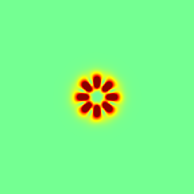

The (squared) error in the gradient field

4. Can we understand this pattern?

According to the gradient theorem it is well known that the integral of the $\nabla a$ field along a closed curve in the domain will be zero. Imagine such a curve consisting of straight-line segments going from cell center to a neighbor-cell center via a face center. If we estimate the contribution of such a segment (of length $\Delta$) to this integral by multiplying in length with the corresponding face gradient our total integral estimate will exatly be zero. However, if we repeat this exersize with analytical face-averaged-gradient values we (gernally) not get zero. As such, the analytical face-averaged gradients can be associated with some “pseudo rotation” ($\omega_p$), which cannot be represented by our discretized solution. The shortest non-zero closed-line “curve” encompasses a single vertex. We can define $\omega_p$ in such a vertex at coordinate $\{x,y\}$,

$\displaystyle \omega_p = -\frac{\int_{x-\Delta}^x \partial_y a \mathrm{d}x + \int_x^{x+\Delta} \partial_y a \mathrm{d}x - \int_{y}^{y + \Delta} \partial_x a \mathrm{d}y + \int_{y-\Delta}^y \partial_x a \mathrm{d}x}{\Delta}.$

  scalar omega[], omg[], psi[];
  vertex scalar omgp[];
  face vector ga[];
  foreach_face()
    ga.x[] = Gauss6_x(x, y, Delta, gradient_2D_x);
  foreach_vertex() {
    omgp[] = (ga.y[] - ga.x[] - ga.y[-1] + ga.x[0, -1])/(Delta);
  }
  foreach() {
    omega[] = -(omgp[] + omgp[1] + omgp[0,1] + omgp[1,1])/4.;
    psi[] = 0;
  }
  output_ppm (omega, file = "omega.png", n = 300, map = blue_white_red);

The pseudo rotation of the analytical solution discretized on faces

The (2D) error vector field ($\vec{F}_e$) statisfies the appropiriate discretization of,

$\displaystyle \nabla \times \vec{F}_e = \omega_p \vec{e}_z.$

Further, since the numerical gradients statisfy the Poisson problem exactly, we know that,

$\displaystyle \nabla \cdot \vec{F}_e = 0,$

And hence we can introduce a Pseudo vector potential $\psi_p$ ($\vec{F}_e = \nabla \times \psi_p\vec{e}_z$) which gives us a Poisson equation for the error vector field,

$\displaystyle \nabla \cdot \nabla \psi_p = -\omega_p$

  TOLERANCE = 1e-15;
  poisson (psi, omega);
  // Computed centered error vector field
  face vector Fe1[];
  vector Fe2[], Fe3[];
  struct { double x, y; } f = {-1.[0],1.[0]};
  foreach_face() 
    Fe1.x[] = face_gradient_x(a,0) - Gauss6_x(x, y, Delta, gradient_2D_x);
  foreach() {
    foreach_dimension() {
      Fe2.x[] = (Fe1.x[] + Fe1.x[1])/2.;
      Fe3.x[] = f.x*(psi[1,1] + psi[-1,1] - psi[1,-1] - psi[-1,-1])/(4.*Delta);
    }
  }
  printf ("%g %g\n", statsf(Fe2.x).max, statsf(Fe2.y).max); // Diagnosed errors
  printf ("%g %g\n", statsf(Fe3.x).max, statsf(Fe3.y).max); // Predicted errors from analytical solution
  vorticity (Fe2, omg); //Circulation of the diagnosed error field
  // Zoom  
  view (fov = 3);
  translate (x = -1, y = -1) {
    squares ("omg", map = blue_white_red);
    vectors ("Fe2", scale = 35, lw = 2);
  }
  save ("Fe2.png");
  translate (x = -1, y = -1) {
    squares ("omega", map = blue_white_red);
    vectors ("Fe3", scale = 35, lw = 2);
  }
  save ("Fe3.png");

We zoom in on the error vectorfield ($\vec{F}_e$) and its rotation.

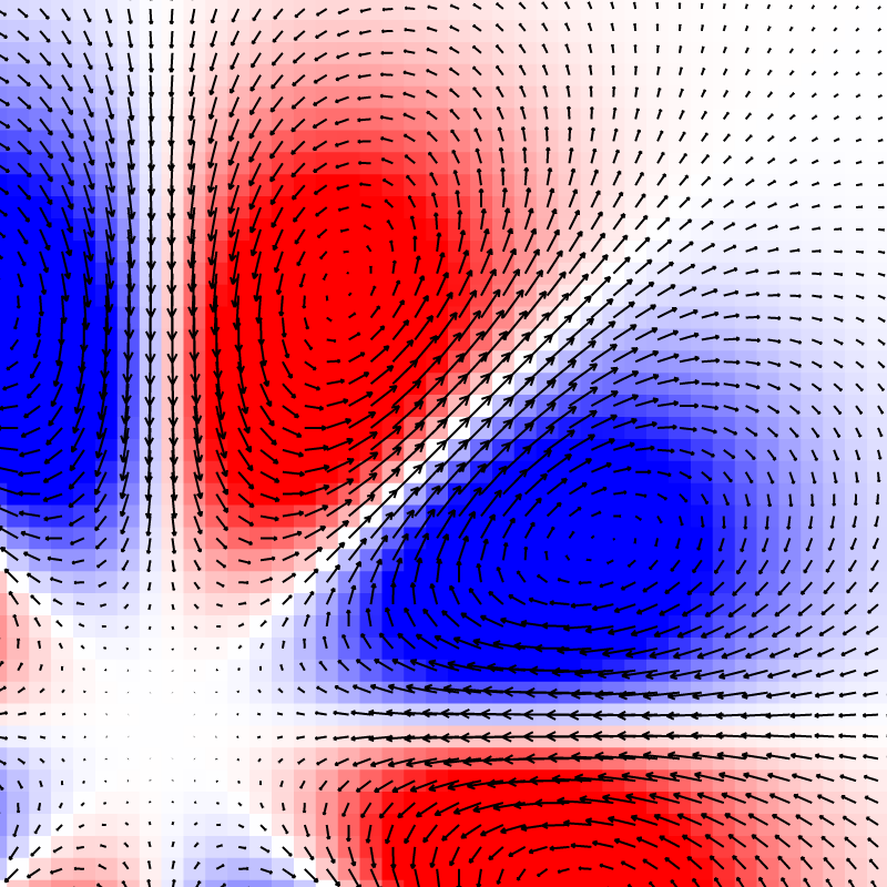
The errors in the solution are associated with vortices

Next, we compare the “expected” error based on the analysis and the analytical solution,

It appears that the “expected error” vector field matches the diagnosed one.

5. An a posteriori error-source estimate

Sofar, we have used the analytical solution for our analysis. In practical applications this is not available. However, one can estimate $\omega_p$ from the solution.

  vector gac[];
  foreach()
    foreach_dimension()
      gac.x[] = (a[1] - a[-1])/(2.*Delta);
  foreach()
    if (sq(x) + sq(y) < sq(4)) //away from boundaries 
      omega[] = (gac.y[2] - gac.y[-2] - gac.x[0,2] + gac.x[0,-2])/(4*Delta);
  output_ppm (omega, file = "aposteriori.png", n = 300);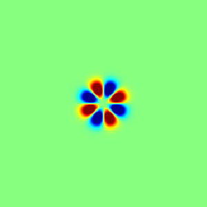

The estimated error source seems to capture its structure correctly

}

See also

• 4th-order accurate error correction