my_second_MG_solver.c

An adaptive solver in space and time

An adaptive solver in space and time

#include "poisson.h"
#include "utils.h"
#include "view.h"

The so-called one-dimensional diffusion equation,

\displaystyle \frac{\partial c}{\partial t} = D\frac{\partial ^2 c}{\partial x^2},

clearly has a two-dimensinal solution space; \{x,t\}. As such, we solve it on a 2D grid. Furthermore, the linearity of the equation motives to use a multigrid approach. Consider the following discretization where timestep (dt) and grid-size (dx) are both denoted with quadtree-grid size \Delta. Such that the area of the a cell has units: length \times time.

\displaystyle \frac{c[0] - c[0,-1]}{\Delta} - D\frac{c[1]-2c[0]+c[-1]}{\Delta^2} = 0.

The residual function then reads:

double D;
static double residual_diff (scalar * al, scalar * bl, scalar * resl, void * data) {
  double maxres = 0;
  scalar a = al[0], res = resl[0];
  foreach (reduction(max:maxres)) {
    res[] = (a[] - a[0,-1])/Delta - D*(a[1] - 2*a[] + a[-1])/(sq(Delta));
    if (fabs(res[]) > maxres)
      maxres = fabs(res[]);
  }
  return maxres;
}

Supplemented with a corresponding relaxation function:

static void relax_diff (scalar * al, scalar * bl, int l, void * data) {
  scalar a = al[0];
  scalar b = bl[0];
  foreach_level_or_leaf(l) {
    double pf = 1./Delta + D*2./sq(Delta);
    a[] = (-b[] + a[0,-1]/Delta + D*(a[1] + a[-1])/sq(Delta))/pf ; 
  }
}

A Multigrid solver function is defined using these functions and the MG cycle.

struct One_D_diffusion {
  scalar a, b;
  (const) face vector alpha;
  (const) scalar lambda;
  double tolerance;
  int nrelax, minlevel;
  scalar * res;
};

mgstats one_D_diffusion (struct One_D_diffusion p) {
  double defaultol = TOLERANCE;
  if (p.tolerance)
    TOLERANCE = p.tolerance;
  scalar a = p.a, b = p.b;
  mgstats s = mg_solve ({a}, {b}, residual_diff, relax_diff,
			&p, p.nrelax, p.res, minlevel = max(1, p.minlevel));
  if (p.tolerance)
    TOLERANCE = defaultol;
  return s;
}

This provides us with the tools to solve the system, provided there are suitable boundary conditions. Notice that the bottom boundary condition now corresponds to the initial condition. We use c(x,0) = sin(2\pi x) and prescribe periodicity of the solution in the x direction, with x \in \{0, 1\}.

scalar c[];
#define SOL (exp(-sq(2*pi*sqrt(D))*y)*(cos(2*pi*(x - Delta/2.)) - cos(2*pi*(x + Delta/2.)))/Delta)  
c[bottom] = dirichlet (SOL);

int main() {
  D = 0.1;
  periodic (left);
  init_grid (8);
  do {
    one_D_diffusion (c);
    boundary ({c});
  } while (adapt_wavelet ({c}, (double[]){0.02}, 8).nf);
   
  view (fov = 10, sy = 0.5, ty = -0.25, tx = -0.5, width = 512, height = 256);
  squares("c");
  cells();
  save("c.png");

The resulting solution and spatio-temporal discretization looks like this:

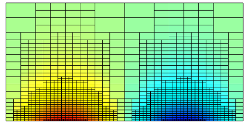
The resulting approximate soluion and grid

Note that at a given time (y), the timestep dy varies within the spatial domain.

The results can be compared against the analytical solution:

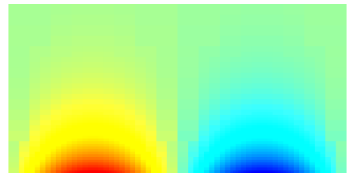
The analytical solution compares well

  foreach()
    c[] = SOL;
  boundary ({c});
  squares ("c");
  save ("sol.png");
}